Week 8 - Simulating Cyclone separator with Discrete Phase Modelling

AIM :

To perform simulation on the cyclone separator using discrete phase modelling, and calculate the separator efficiency and pressure drop.

OBJECTIVES :

• To import the given cyclone separator model into spaceclaim and extract the fluid volume.
• To generate mesh for the fluid volume by choosing the mesh method as cartesian which provides the structural mesh with mesh element size as 5 mm.
• To setup the discrete phase model for the simulation with various particles size and velocities, and compare the separator efficiency and pressure drop for those cases.
• To post process the results.

INTRODUCTION :

The main objective of this simulation is to find the efficiency of the cyclone seperator for the same particle velocity of 3 m/s for the various particle size such as 1e-6m, 3e-6m and 5e-6m and compare the results. Then, by keeping the particle size of 5e-6m as constant, vary the velocity of the particle and fluid as 1,3 and 5m/s and compare the results. Here, we are using discrete phase modelling for tracking the particles in the separator and since the particle size is so small, the particle interaction with the continuous flow fluid (air) option is enabled.

Cyclone separator :

The cyclone separators are the seperation devices which seperate the particulate matter from the flue gas. They use the principle of inertia to seperate the particles from the flue gas. These are utilised in many applications due to their low cost, simple design and high efficiency.

• `"Separator efficiency, "eta = "Number of particles trapped at the bottom outlet" / "Total number of particles tracked"`

Working of cyclone separator :

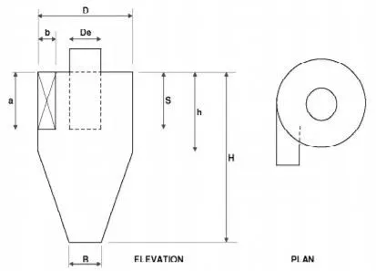
Cyclone separators work much like a centrifuge, but with a continuous feed of dirty air. In a cyclone separator, dirty flue gas is fed into a chamber. The inside of the chamber creates a spiral vortex, similar to a tornado. This spiral formation and the separation is shown in Figure . The lighter components of this gas have less inertia, so it is easier for them to be influenced by the vortex and travel up it. Contrarily, larger components of particulate matter have more inertia and are not as easily influenced by the vortex.Since these larger particles have difficulty following the high-speed spiral motion of the gas and the vortex, the particles hit the inside walls of the container and drop down into a collection hopper. These chambers are shaped like an upside-down cone to promote the collection of these particles at the bottom of the container. The cleaned flue gas escapes out the top of the chamber.

Empirical models used to calculate the cyclone separator efficiency :

1. IOZIA AND LEITH MODEL:

Iozia and Leith (1990) logistic model is a modified version of Barth (1956) model which is developed based on force balance. The model assumes that a particle carried by the vortex endures the influence of two forces: a centrifugal force,

Z, and a flow resistance, W. Core length, zc, and core diameter ,dc are given as:

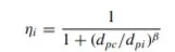
β is an expression for slope parameter derived based on the statistical analysis of experimental data of a cyclone with D = 170

0.25 m given as:

and dpc is the 50% cut size given by Barth:

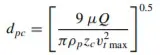
where core length, zc, and core diameter, dc, are given as,

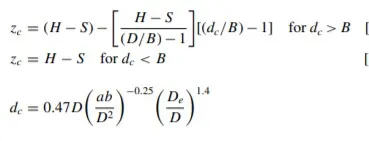
2. LI AND WANG MODEL:

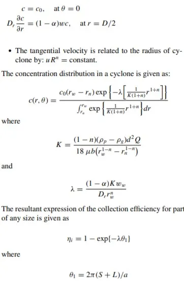
The Li and Wang [3] model includes particle bounce or reentrainment and turbulent diffusion at the cyclone wall. A twodimensional analytical expression of particle distribution in the cyclone is obtained. Li and Wang model was developed based 180 on the following assumptions:

The radial particle velocity and the radial concentration profile are not constant for uncollected particles within the cyclone.

Boundary conditions with the consideration of turbu185 lent diffusion coefficient and particle bounce reentrainment on the cyclone wall are:

3. KOCH AND LICHT MODEL:

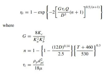
Koch and Licht [2] collection theory recognized the inherently turbulent nature of cyclones and the distribution of gas residence times within the cyclone. Koch and Licht described particle motion in the entry and collection regions with the ad- 200 ditional following assumptions:

• The tangential velocity of a particle is equal to the tangential velocity of the gas flow, i.e. there is no slip in the tangential direction between the particle and the gas.
• The tangential velocity is related to the radius of cy- 205 clone by: u Rn = constant.

A force balance and an equation on the particles collection yields the grade efficiency ηi:

4. LAPPLE MODEL:

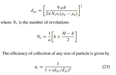
Lapple [1] model was developed based on force balance without considering the flow resistance. Lapple assumed that a par215 ticle entering the cyclone is evenly distributed across the inlet opening. The particle that travels from inlet half width to the wall in the cyclone is collected with 50% efficiency. The semi empirical relationship developed by Lapple [1] to calculate a 50% cut diameter, dpc, is:

• The collection efficiency of cyclones varies as a function of density, particle size and cyclone design.
• Cyclone efficiency will generally increase with increases in particle size and/or density, inlet duct velocity, cyclone body length, number of gas revolutions in the cyclone, ratio of cyclone body diameter to gas exit diameter, inlet dust loading, smoothness of the cyclone inner wall. Similarly, cyclone efficiency will decrease with increases in the parameters such as gas viscosity, cyclone body diameter, gas exit diameter, gas inlet duct area, gas density, leakage of air into the dust outlet.
• The pressure drop is a function of the inlet velocity and cyclone diameter. Form the above discussion it is clear that small cyclones are more efficient than large cyclones. Small cyclones, however, have a higher pressure drop and are limited with respect to volumetric flow rates. Another option is arrange smaller cyclones in series and/or in parallel to substantially increase efficiency at lower pressure drops. These gains are somewhat compensated, however, by the increased cost and maintenance problems. Also these types of arrangements tend to plug more easily. When common hoppers are used in such arrangements, different flows through cyclones can lead to reentrainment problems.

CASE SETUP :

The simulations are performed for various cases which are shown below,

	MESH ELEMENT SIZE (in 'mm')	NUMBER OF MESH ELEMENTS (Cartesian)	VELOCITY (in 'm/s')	PARTICLE SIZE (in `mum`)
CASE 1	5	427871	1	3
CASE 2	5	427871	3	3
CASE 3	5	427871	5	3
CASE 4	5	427871	5	1
CASE 5	5	427871	5	5

• For this simulation, we generate structured mesh by inserting the cartesian method. This gives the best results for the simulation. Also, the number of mesh cells in the inlet of the separator gives the total number of particles to be tracked.
• Here, since the swirl flow dominates because of the geometry of the separator, we choose the k-epsilon RNG turbulence model with swirl dominated flow option enabled. This provide more accurate simulation results compared to others.
• The material of the discrete particle is taken as anthracite which is a hard variety of coal.

PROCEDURE :

CASE - 1 (for particle size as 1e-6m and velocity 3 m/s) :

PRE-PROCESSING :

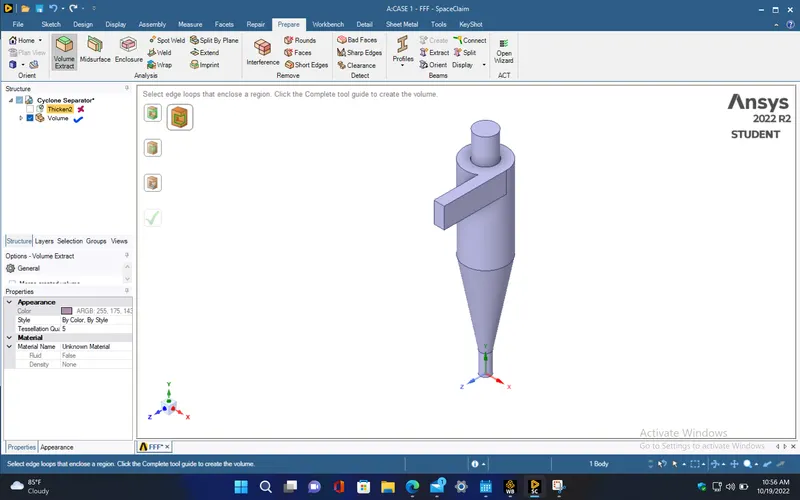
• Import the given cyclone separator model into spaceclaim and extract its fluid volume using Volume Extract option under Prepare menu.

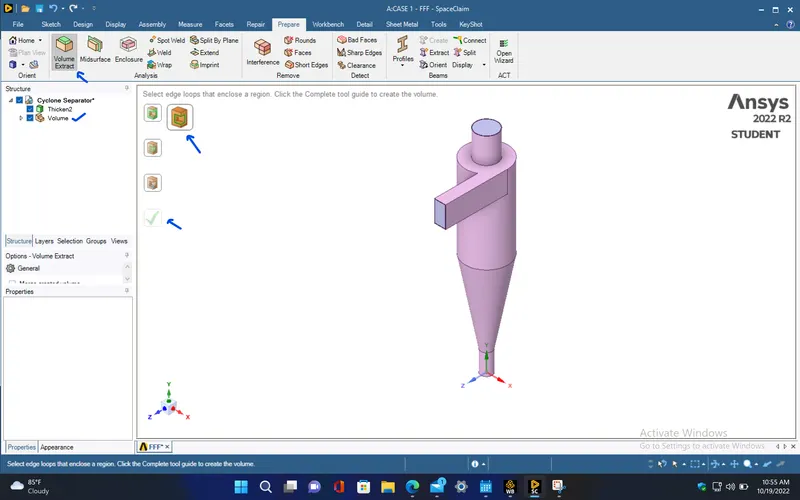
• Hide and suppress the outer solid volume of the cyclone separator in order to perform the simulation only on the fluid volume. Then, close the spaceclaim.

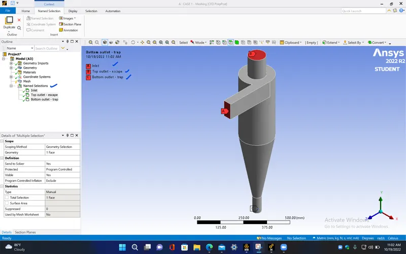
• Now, open the mesh window from the Ansys standalone workflow and give names for the required regions of the cyclone separator fluid volume.

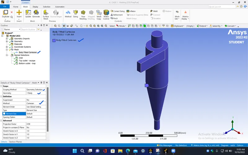
• Insert a new mesh method and choose the method as cartesian for the body. This will generate the structured hexahedral mesh.

• Give the element size as 5mm and generate the mesh.

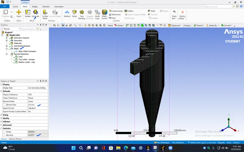
• Since it is the structured mesh, the element quality is high for almost every mesh elements.

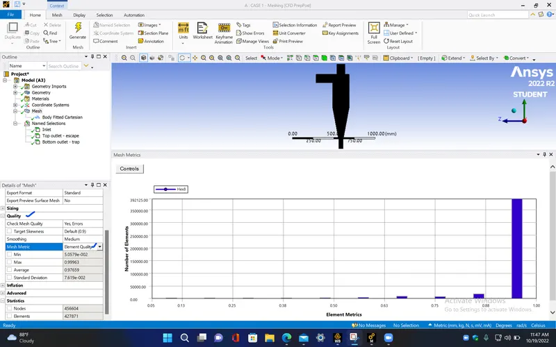
• The number of particles entering the inlet of the cyclone separator can be tracked by finding the number of mesh cells at inlet.

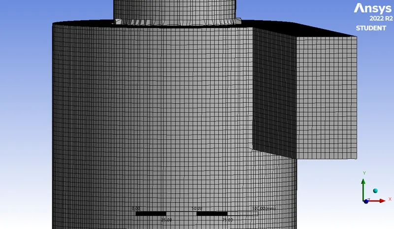
• Cross sectional view,

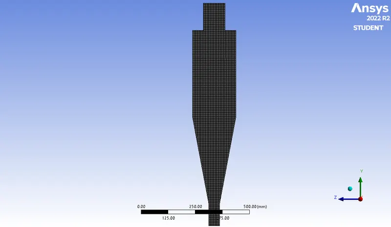
Cells	Faces	Nodes
427871	1312260	456604

SETUP AND SOLVING :

• Give the following parameters for the simultion.

Model	Settings
Space	3D
Time	Steady
Viscous	RNG k-epsilon turbulence model

Wall Treatment	Standard Wall Functions
RNG Swirl Dominated Flow Option	Enabled
Coupled Dispersed Phase	Enabled

Material properties :

Fluid	air
Density	1.225 kg/m^3
Cp (Specific Heat)	1006.43 J/(kg K)
Thermal Conductivity	0.0242 W/(m K)
Viscosity	1.7894e-05 kg/(m s)
Molecular Weight	28.966 kg/kmol

Boundary conditions :

inlet
Velocity Specification Method	Magnitude, Normal to Boundary
Reference Frame	Absolute
Velocity Magnitude [m/s]	3
Discrete Phase BC Type	reflect
top_outlet_-_escape
Backflow Reference Frame	Absolute

Gauge Pressure [Pa]	0
Backflow Direction Specification Method	Normal to Boundary
Discrete Phase BC Type	escape
bottom_outlet_-_trap
Backflow Reference Frame	Absolute
Gauge Pressure [Pa]	0
Backflow Direction Specification Method	Normal to Boundary
Discrete Phase BC Type	trap
wall-volume_volume
Wall Motion	Stationary Wall
Shear Boundary Condition	No Slip
Discrete Phase BC Type	reflect

Solution method :

Pressure-Velocity Coupling	Coupled
Pseudo Time Method (Global Time Step)	True
Discretization Scheme
Pressure	Second Order
Momentum	Second Order Upwind
Turbulent Kinetic Energy	Second Order Upwind
Turbulent Dissipation Rate	Second Order Upwind

• Here, the gravity is enabled since the particles are to be trapped at the bottom of the cyclone separator. The gravitational acceleration is towards the negative y-axis direction of the cyclone separator. So, the gravity acceleration is given on the required axis direction.

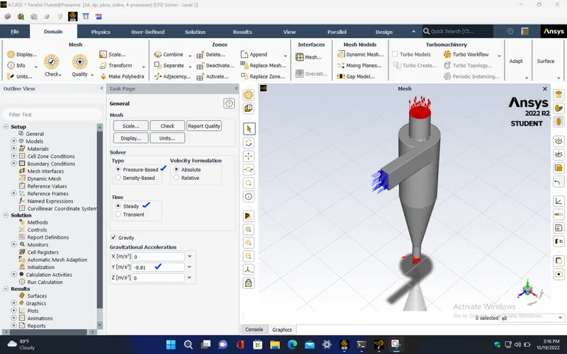
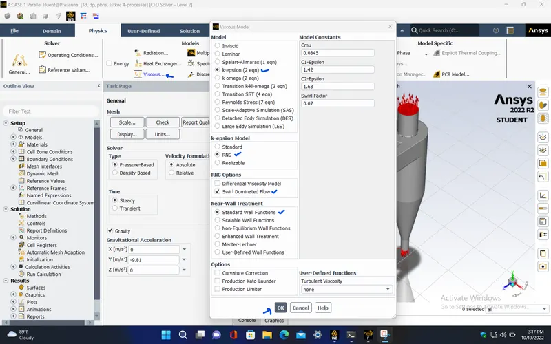
• Here, the k-epsilon RNG turbulence model is chosen as the viscous model with swirl dominated flow option enabled. Since the simulation is performed mainly to track the discrete particles which are flowing along with fluid(air) having the high swirling effect, the k-epsilon RNG turbulence model will be the correct choice for this model.

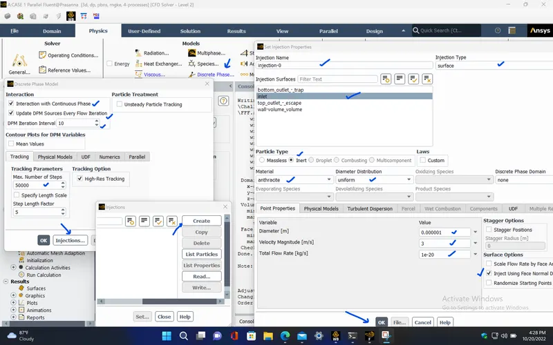
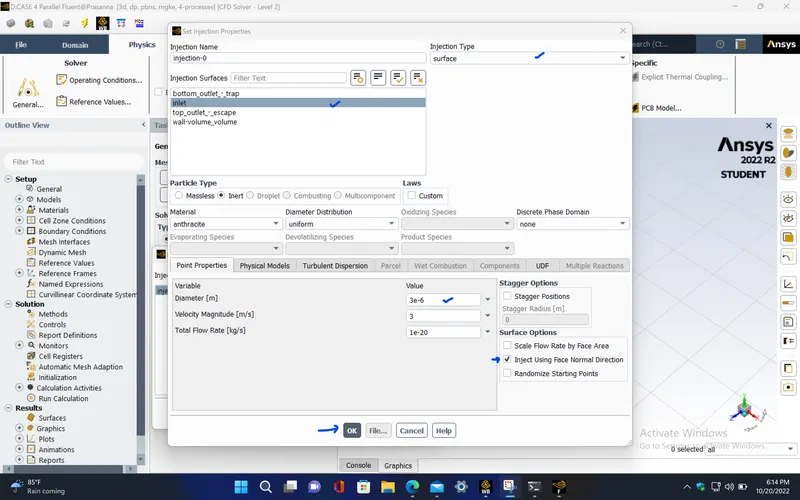
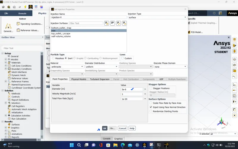
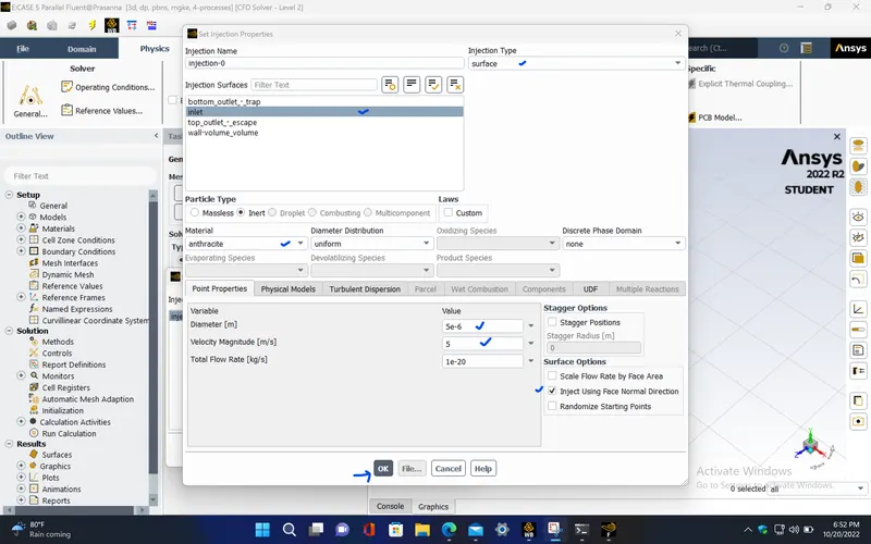
• Enable the discrete phase model. Create the injection of particles by selecting the injection type as surface from inlet and the particles material as anthracite. Then, give the particle diameter as 1*e-6 m and velocity in the normal direction of the inlet surface as 3 m/s .

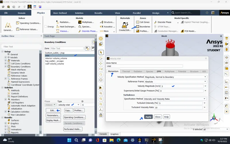
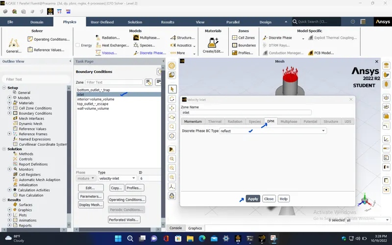
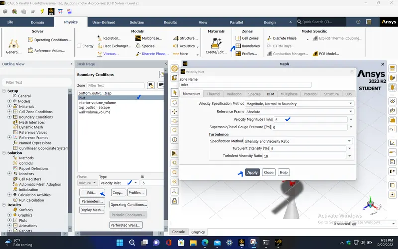
• Give the inlet velocity of the fluid(air) as 3 m/s and under DPM, select the discrete phase BC type as reflect.

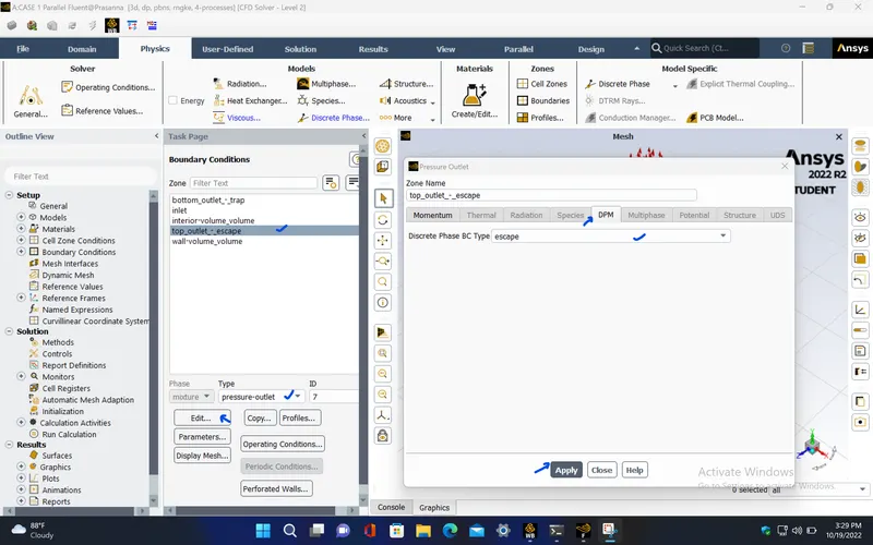
• Give the boundary conditions for the top outlet as pressure outlet with atmospheric pressure and give the discrete phase BC type as escape.

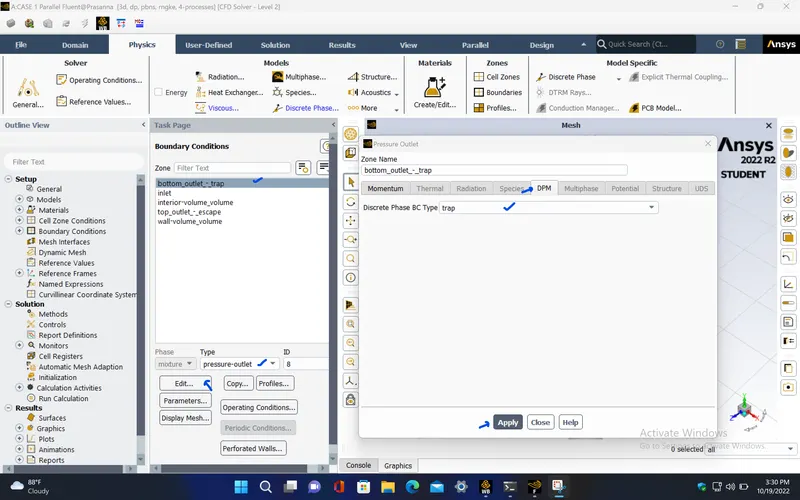
• Give the boundary conditions for the bottom outlet as pressure outlet with atmospheric pressure and give the discrete phase BC type as trap since the particles are to be trapped here.

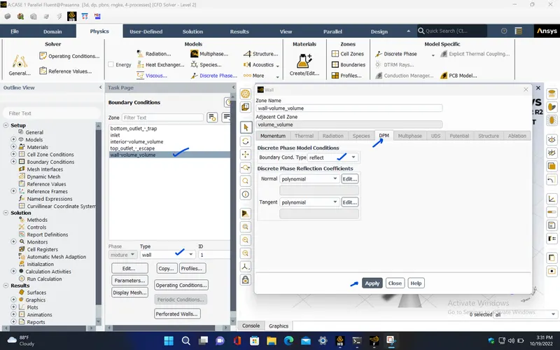
• For the wall, check if the DPM is a given as reflect.

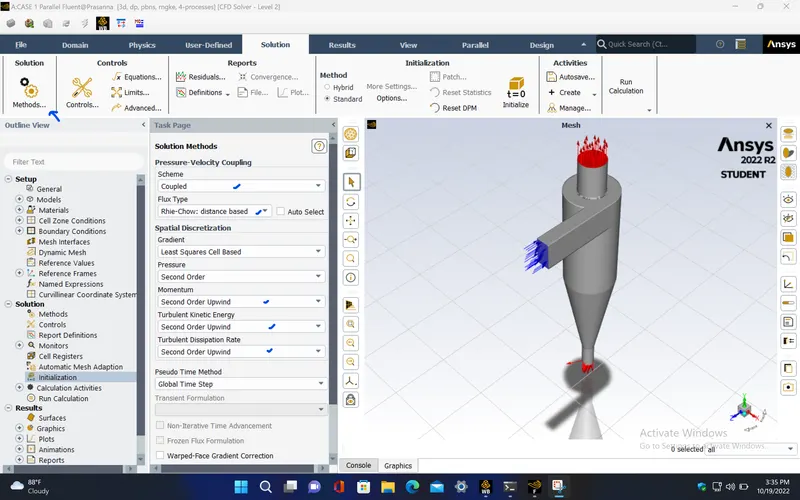
• In order to track the discrete particles more accurately, select the second order upwind for both turbulent kinetic energy and dissipation rate under spatial discretization. Here, select the scheme as coupled for the pressure velocity coupling.

• Initialize the simulation using standard initialization and select compute from inlet option.

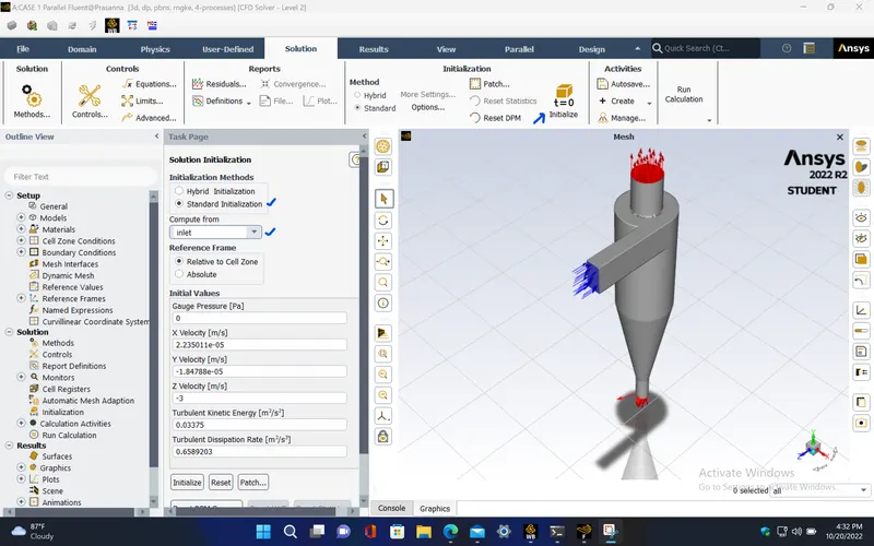
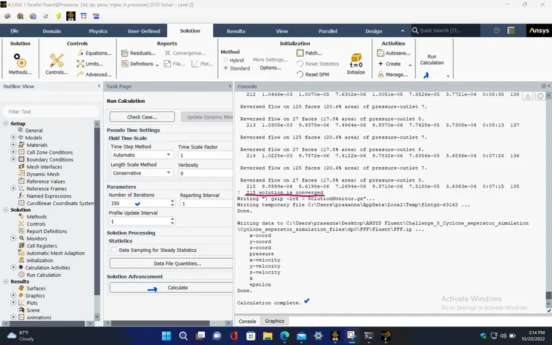
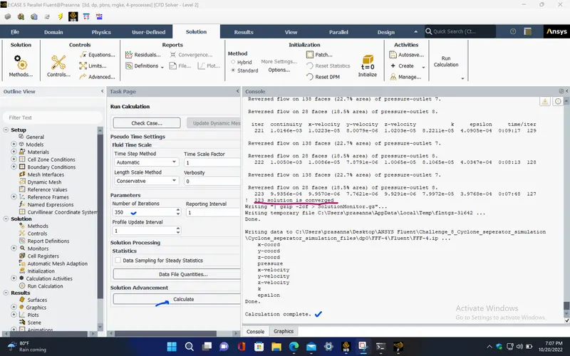
• Run the simulation for 350 iterations.

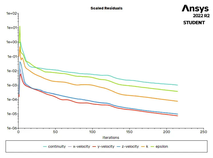
RESIDUALS PLOT :

Solution status :

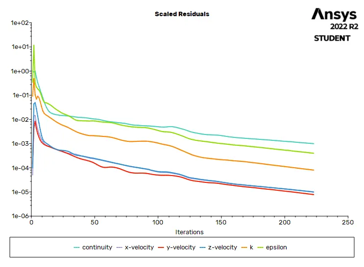
• From the above plots, we see that the solution got converged at 215th iteration since the rate at which residuals change becomes constant over iteration.

Number of iterations : 215

	Value	Absolute Criteria	Convergence Status
continuity	0.0009899933	0.001	Converged
x-velocity	9.619775e-06	0.001	Converged
y-velocity	7.269354e-06	0.001	Converged
z-velocity	9.571005e-06	0.001	Converged
k	7.518043e-05	0.001	Converged
epsilon	0.0003636262	0.001	Converged

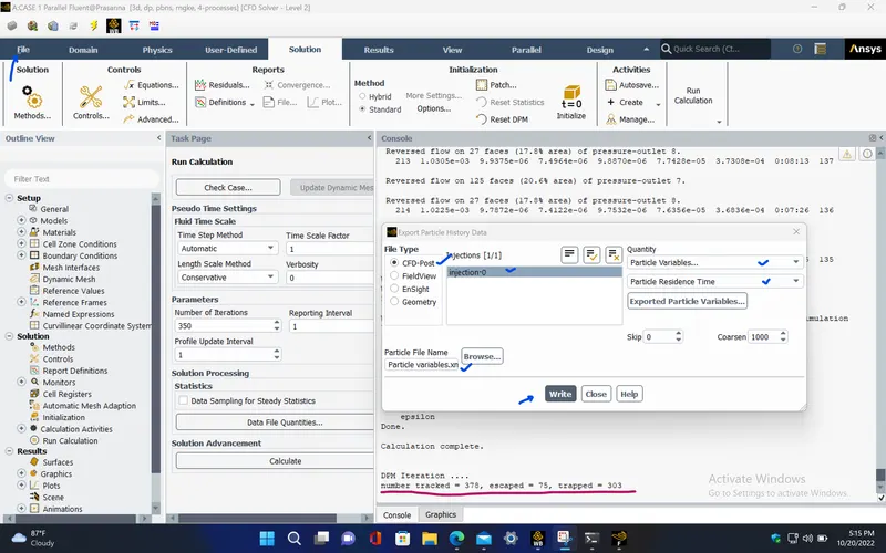
• Total number of particles tracked = 378
• Number of particles escaped through top outlet = 75
• Number of particles trapped into bottom outlet = 303

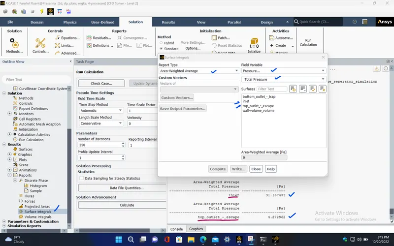
• Total pressure at the inlet = 31.167 (in 'Pa')
• Total pressure at the top outlet = 4.273 (in 'Pa')

POST PROCESSING :

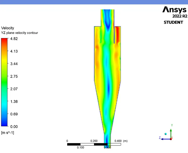
VELOCITY CONTOUR (YZ plane) :

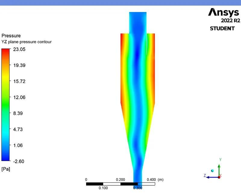
PRESSURE CONTOUR (YZ plane) :

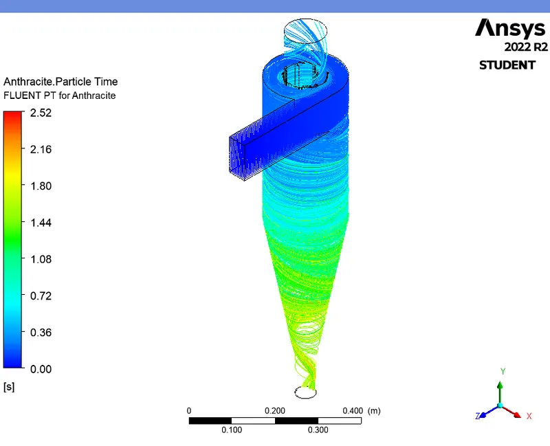
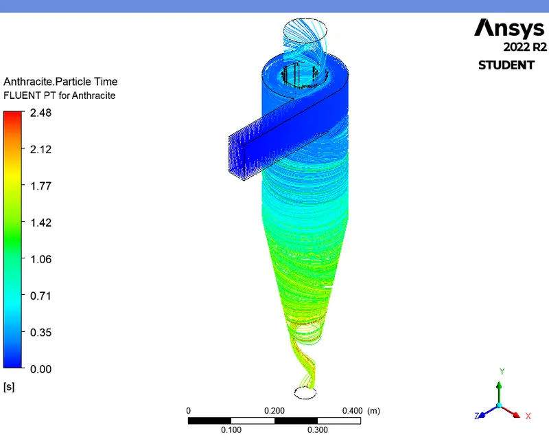
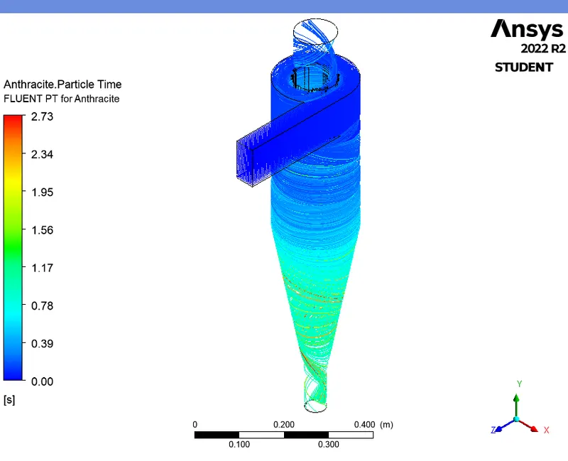
ANTHRACITE PARTICLES TIME :

CASE - 2 (for particle size as 3e-6m and velocity 3 m/s) :

• Here, change the particle size to 3*e-6m and repeat the same steps as the discussed in the previous case.

RESIDUALS PLOT :

Solution status :

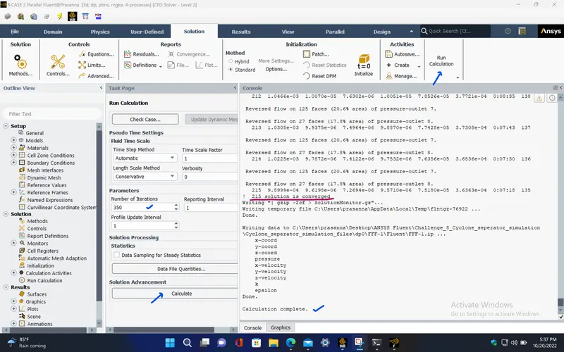
• From the above plots, we see that the solution got converged at 215th iteration since the rate at which residuals change becomes constant over iteration.

Number of iterations : 215

	Value	Absolute Criteria	Convergence Status
continuity	0.0009899933	0.001	Converged
x-velocity	9.619775e-06	0.001	Converged
y-velocity	7.269354e-06	0.001	Converged
z-velocity	9.571005e-06	0.001	Converged
k	7.518043e-05	0.001	Converged
epsilon	0.0003636262	0.001	Converged

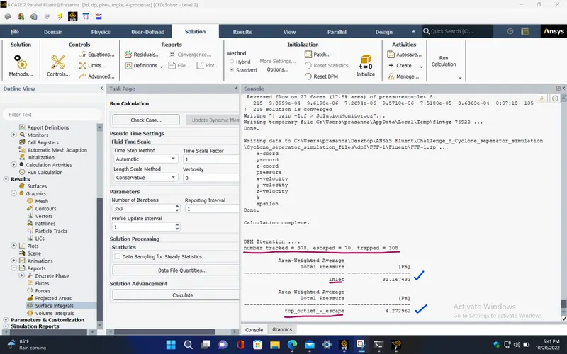
• Total number of particles tracked = 378
• Number of particles escaped through top outlet = 70
• Number of particles trapped into bottom outlet = 308
• Total pressure at the inlet = 31.167 (in 'Pa')
• Total pressure at the top outlet = 4.273 (in 'Pa')

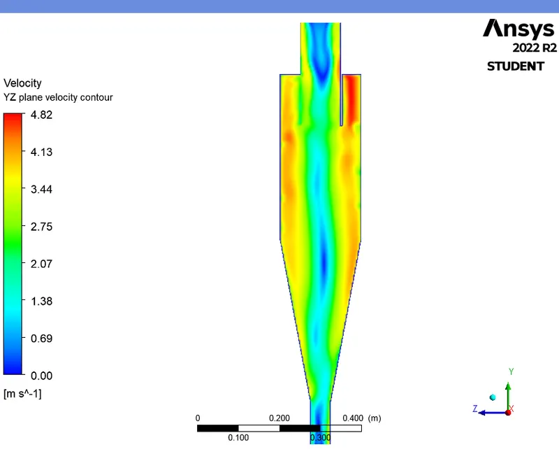
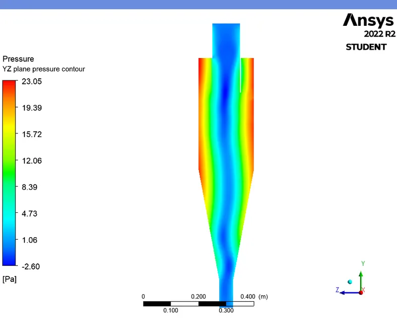
VELOCITY CONTOUR (YZ plane) :

PRESSURE CONTOUR (YZ plane) :

ANTHRACITE PARTICLES TIME :

CASE - 3 (for particle size as 5e-6m and velocity 3 m/s) :

• Here, change the particle size to 5*e-6m and repeat the same steps as the discussed in the previous case.

RESIDUALS PLOT :

Solution status :

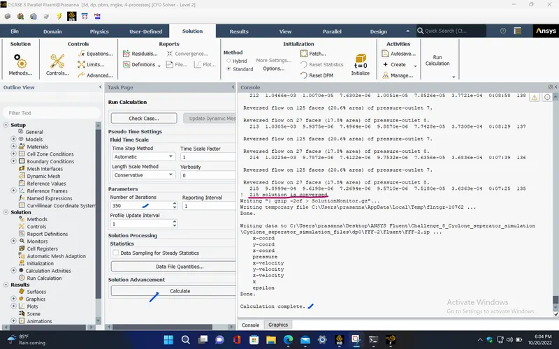
• From the above plots, we see that the solution got converged at 215th iteration since the rate at which residuals change becomes constant over iteration.

Number of iterations : 215

	Value	Absolute Criteria	Convergence Status
continuity	0.0009899933	0.001	Converged
x-velocity	9.619775e-06	0.001	Converged
y-velocity	7.269354e-06	0.001	Converged
z-velocity	9.571005e-06	0.001	Converged
k	7.518043e-05	0.001	Converged
epsilon	0.0003636262	0.001	Converged

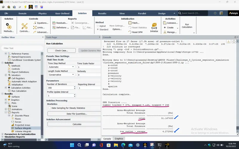
• Total number of particles tracked = 378
• Number of particles escaped through top outlet = 133
• Number of particles trapped into bottom outlet = 245
• Total pressure at the inlet = 31.167 (in 'Pa')
• Total pressure at the top outlet = 4.273 (in 'Pa')

VELOCITY CONTOUR (YZ plane) :

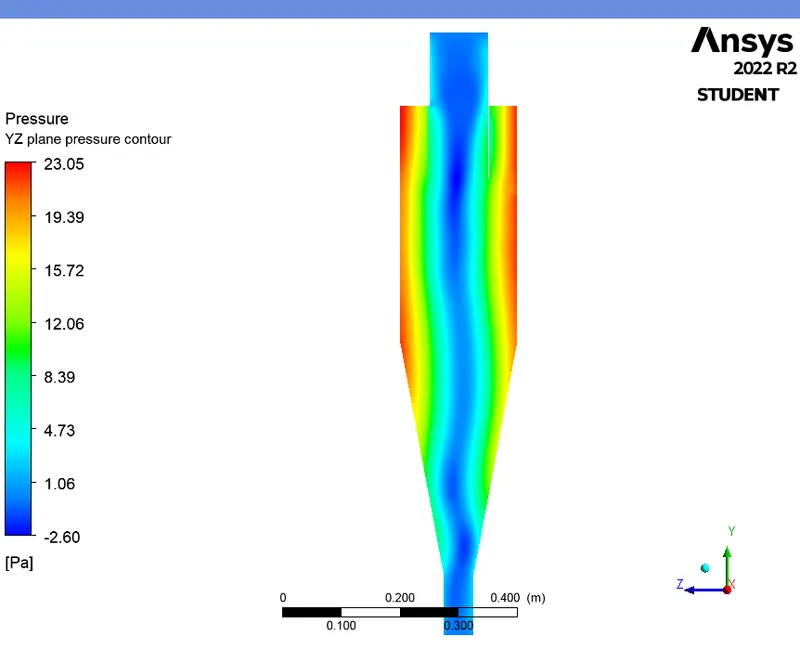
PRESSURE CONTOUR (YZ plane) :

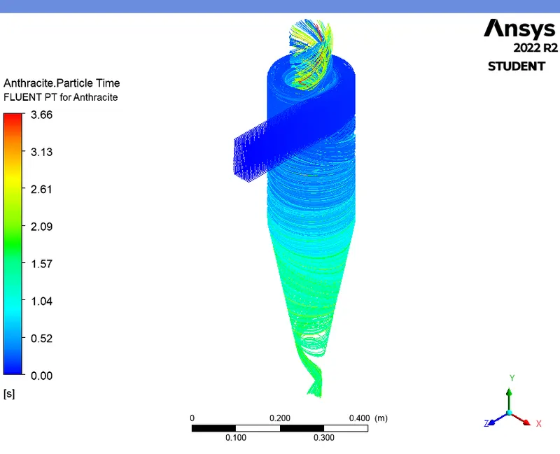
ANTHRACITE PARTICLES TIME :

CASE - 4 (for particle size as 5e-6m and velocity 1 m/s) :

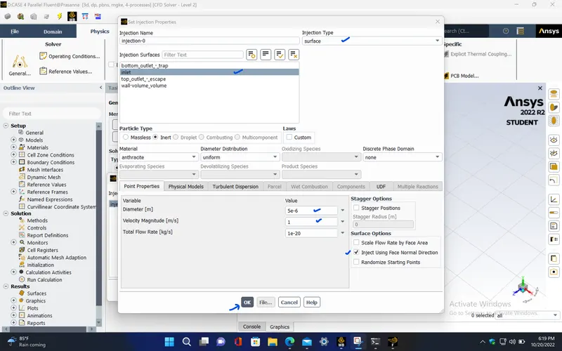
• Here, change the velocity to 1 m/s for the same particle size of 5*e-6m and repeat the same steps as the discussed in the previous case.

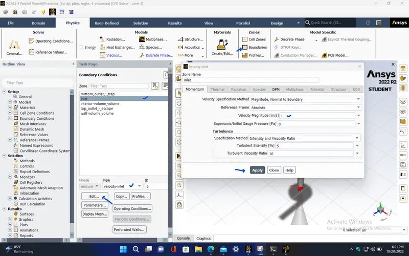
Boundary conditions :

inlet
Velocity Specification Method	Magnitude, Normal to Boundary
Reference Frame	Absolute
Velocity Magnitude [m/s]	1
Discrete Phase BC Type	reflect
top_outlet_-_escape
Backflow Reference Frame	Absolute

Gauge Pressure [Pa]	0
Backflow Direction Specification Method	Normal to Boundary
Discrete Phase BC Type	escape
bottom_outlet_-_trap
Backflow Reference Frame	Absolute
Gauge Pressure [Pa]	0
Backflow Direction Specification Method	Normal to Boundary
Discrete Phase BC Type	trap
wall-volume_volume
Wall Motion	Stationary Wall
Shear Boundary Condition	No Slip
Discrete Phase BC Type	reflect

RESIDUALS PLOT :

Solution status :

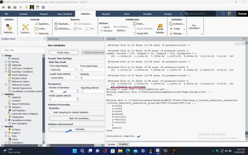
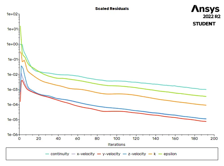
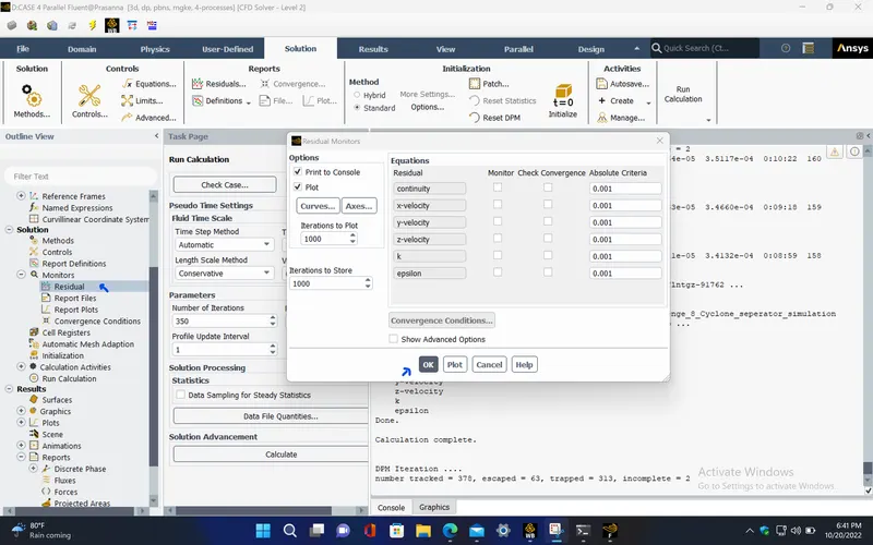
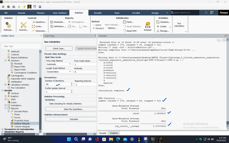
• From the above plots, we see that the solution got converged at 192th iteration since the rate at which residuals change becomes constant over iteration. But, since two particles are trapped inside the separator, the simulation is set to run for fewer more iteration.

Number of iterations : 192 (solution converged) + 28 = 220

	Value	Absolute Criteria	Convergence Status
continuity	0.0006597259	0.001	Converged
x-velocity	6.908232e-06	0.001	Converged
y-velocity	4.693745e-06	0.001	Converged
z-velocity	6.99741e-06	0.001	Converged
k	5.55877e-05	0.001	Converged
epsilon	0.0002101891	0.001	Converged

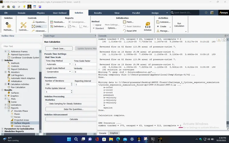
• Total number of particles tracked = 378
• Number of particles escaped through top outlet = 66
• Number of particles trapped into bottom outlet = 312
• Total pressure at inlet = 2.85585 (in 'Pa')
• Total pressure at top outlet = 0.37578 (in 'Pa')

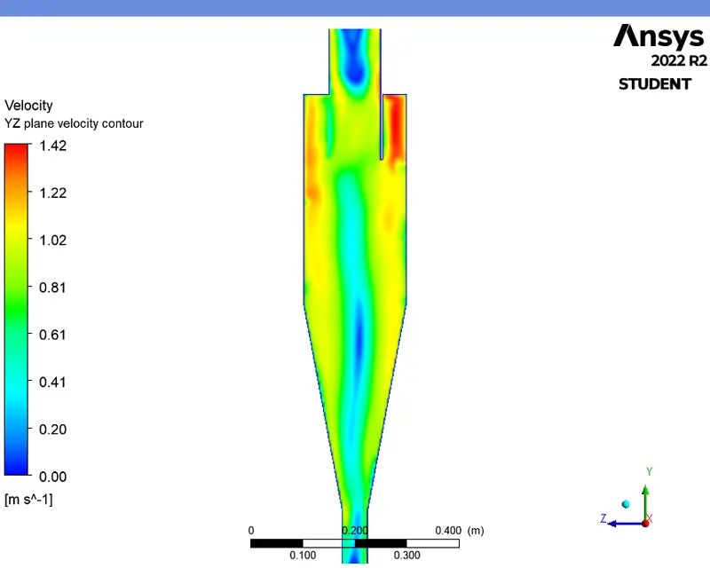
VELOCITY CONTOUR (YZ plane) :

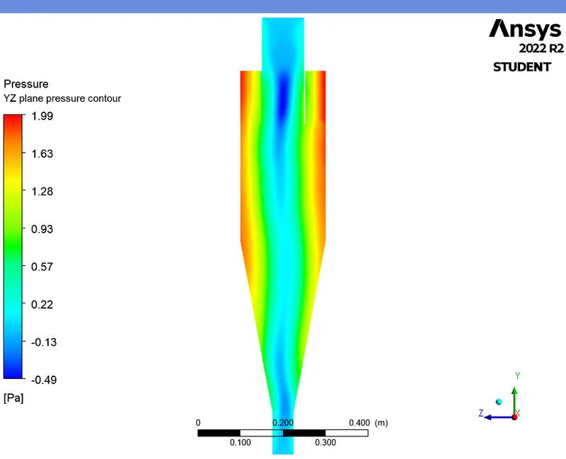
PRESSURE CONTOUR (YZ plane) :

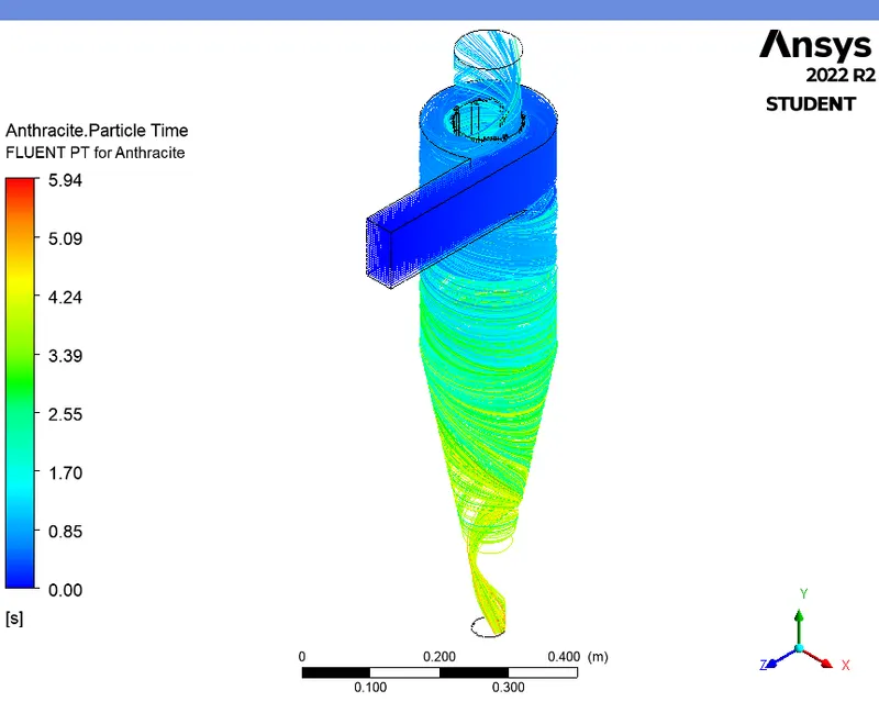
ANTHRACITE PARTICLES TIME :

CASE - 5 (for particle size as 5e-6m and velocity 5 m/s) :

• Here, change the velocity to 5 m/s for the same particle size of 5*e-6m and repeat the same steps as the discussed in the previous case.

Boundary conditions :

inlet
Velocity Specification Method	Magnitude, Normal to Boundary
Reference Frame	Absolute
Velocity Magnitude [m/s]	5
Discrete Phase BC Type	reflect
top_outlet_-_escape
Backflow Reference Frame	Absolute

Gauge Pressure [Pa]	0
Backflow Direction Specification Method	Normal to Boundary
Discrete Phase BC Type	escape
bottom_outlet_-_trap
Backflow Reference Frame	Absolute
Gauge Pressure [Pa]	0
Backflow Direction Specification Method	Normal to Boundary
Discrete Phase BC Type	trap
wall-volume_volume
Wall Motion	Stationary Wall
Shear Boundary Condition	No Slip
Discrete Phase BC Type	reflect

RESIDUALS PLOT :

Solution status :

• From the above plots, we see that the solution got converged at 215th iteration since the rate at which residuals change becomes constant over iteration.

Number of iterations : 223

	Value	Absolute Criteria	Convergence Status
continuity	0.0009935613	0.001	Converged
x-velocity	9.956981e-06	0.001	Converged
y-velocity	7.76211e-06	0.001	Converged
z-velocity	9.929071e-06	0.001	Converged
k	7.997228e-05	0.001	Converged
epsilon	0.0003976755	0.001	Converged

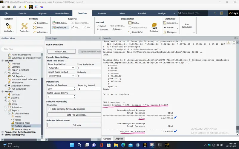
• Total number of particles tracked = 378
• Number of particles escaped through top outlet = 71
• Number of particles trapped into bottom outlet = 307
• Total pressure at the inlet = 89.974 (in 'Pa')
• Total pressure at the top outlet = 12.492 (in 'Pa')

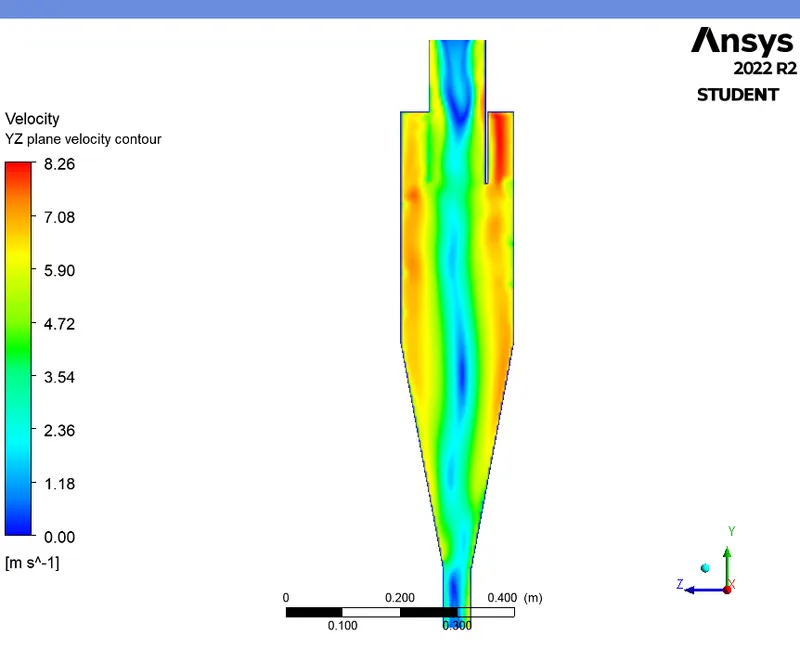
VELOCITY CONTOUR (YZ plane) :

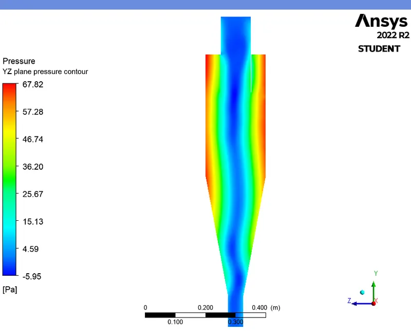
PRESSURE CONTOUR (YZ plane) :

ANTHRACITE PARTICLES TIME :

RESULTS :

Google drive link for the Ansys file,

https://drive.google.com/file/d/1GFBQa82c6FpQx3t4pM7sG3695vHipObI/view?usp=sharing

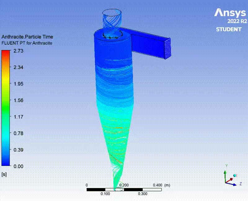
Anthracite particle time animation :

	PARTICLE SIZE `("in " mum)`	VELOCITY (in ‘m/s’)	TOTAL NUMBER OF PARTICLES TRACKED	NUMBER OF PARTICLES ESCAPED THROUGH OUTLET	NUMBER OF PARTICLES INTO BOTTOM OUTLET	SEPARATOR EFFICIENCY, `eta`	PRESSURE DROP (Inlet pressure - Top outlet pressure) (in 'Pascal')
CASE 1	1	3	378	75	303	80.16	26.89
CASE 2	3	3	378	70	308	81.48	26.89
CASE 3	5	3	378	133	245	64.81	26.89
CASE 4	5	1	378	66	312	82.54	2.48
CASE 5	5	5	378	71	307	81.22	77.48

CONCLUSION :

From the above table, we can observe that for the same particle size of 5e-6m, as the velocity increases the efficiency of the separator decreases. This is due to the increase in swirling effect as the velocity increase and hence the number of particles escaped also increases. Also, we can see that, for the same inlet velocity of 3 m/s, as the particle size increases the efficiency also increases (except for case 3). This is because the inertial force on the paticles increases as the particles size increases causing the particles to get trapped at the bottom.

Now, if we observe the pressure drop column in the above table, we can see that, as the velocity of the fluid(air) and particles increases at inlet the pressure drop also increases which causes the some particles to escape through the top outlet.

REFERENCES :

1. https://www.researchgate.net/publication/232747389_A_CFD_Study_on_the_Prediction_of_Cyclone_Collection_Efficiency

2. https://www.sciencedirect.com/science/article/pii/S0307904X06000291