Week 1- Mixing Tee
AIM :
To perform the simulation for steady state flow of the hot air and cold air through the given Short and Long Mixing Tee models using Ansys fluent with different momentum ratio of 2 and 4 for each case, and to compare the mixing effectiveness for those cases.
OBJECTIVES :
- To extract the fluid volume from the given mixing tee models.
- To perform meshing over the fluid domain.
- To provide different boundary conditions by changing the momentum ratio as 2 and 4 for both cases (for short tee and long tee models), and to run the simulations until the solution gets converged.
- To plot the temperature and velocity contours at outlet for each case and to compare the results.
INTRODUCTION :
In this project, we are going to simulate the flow of hot and cold air through Short and Long Mixing Tee in order to find out the temperature and velocity distribution over the fluid domain. Hence, from that, we can find out the mixing effectiveness of the fluid streams over the domain for different mixing tee models and compare the results. Here, we use steady state time study for the flow analysis purpose. Then, the average temperature at outlet which is found by running simulations in Ansys fluent is compared with the analytical solution for verification and validation purpose.
Mixing Tee and its importance:
It is a type of mixing mechanism which is used to mix any two fluid streams flowing perpendicular to each other. In some air conditioning applications, the fresh air from atmosphere is mixed with the cold air by using this mixing tee before the air gets inside the system(i.e, the air conditioned room). This increases the effectiveness of the air conditioner and also comforts the people inside the system.
Momentum ratio :
Momentum ratio (M.R) = velocity at cold inlet (`v_c`) / velocity at hot inlet `(v_h)`
Formula used to find the temperature and velocity at outlet, analytically:
1. From the mass balance equation,
We know that,
`dot m_h + dot m_c = dot m_o`
`rho * A_h * v_h + rho * A_c * v_c = rho * A_o * v_o`
Where,
- `dot m` - mass flow rate of the fluid, in kg/s = `rho * A * v`
- A - Cross sectional area in which the fluid is flowing, in `m^2`
- v - velocity of the fluid, in m/s
`pi/4 * (d_h^2 * v_h + d_c^2 * v_c) = pi/4 * (d_o^2 * v_o)`
`v_o = (d_h^2 * v_h + d_c^2 * v_c) / d_o^2`
- For M.R = 2,
`v_o = (0.0339^2 * 3 + 0.017^2 * 6) / 0.0339^2`
`v_o = 4.50435`m/s
- For M.R = 4,
`v_o = (0.0339^2 * 3 + 0.017^2 * 12) / 0.0339^2`
`v_o = 6.0087` m/s
2. From the energy balance equation,
We know that,
`dot m_h * h_h + dot m_c * h_c = dot m_o * h_o`
Where,
- h - Enthalpy of the fluid, in J = `C_p * T`
- `C_p` - Specific heat of the fluid (air), in J/kg-K
- T - Temperature of the fluid, in K
`C_p(dot m_h * T_h + dot m_c * T_c) = C_p(dot m_o * T_o)`
`T_o = (dot m_h * T_h + dot m_c * T_c) / (dot m_h + dot m_c)`
`T_o = (d_h^2 * v_h * T_h + d_c^2 * v_c * T_c) / (d_h^2 * v_h + d_c^2 * v_c)`
- For M.R = 2,
`T_o = (0.0339^2 * 3 * 36 + 0.017^2 * 6 * 19) / (0.0339^2 * 3 + 0.017^2 * 6)`
`T_o = 30.3224`C
- For M.R = 4,
`T_o = (0.0339^2 * 3 * 36 + 0.017^2 * 12 * 19) / (0.0339^2 * 3 + 0.017^2 * 12)`
`T_o = 27.4877`C
PROBLEM APPROACH :
Here, we divide the given problem into two major cases and for each case, we sub-divide into futher cases for different momentum ratios,
- Case 1
- Short mixing tee with a hot inlet velocity of 3m/s.
- Momentum ratio of 2, 4. (for M.R = 2, cold air inlet velocity is 6 m/s whereas, for M.R = 4, cold air inlet velocity is 12 m/s)
- Case 2
- Long mixing tee with a hot inlet velocity of 3m/s.
- Momentum ratio of 2, 4. (for M.R = 2, cold air inlet velocity is 6 m/s whereas, for M.R = 4, cold air inlet velocity is 12 m/s)
- Steady state time is performed all the cases.
- The number of iterations is taken as 500 for all the cases.
- The mesh element size is taken as 3mm for all the cases except for the mesh independent case studies.
- The k-epsilon turbulence model is chosen for all the cases except for one case where k-epsilon and k-omega are compared (short tee model with M.R - 4 )
PROCEDURE :
1. Case 1 - Short Tee with M.R - 2 :
PRE-PROCESSING :
- Create a fluid flow (fluent) from analysis systems in Ansys workbench and Import the short tee model into the spaceclaim under geometry.
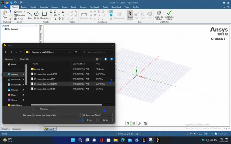
- Extract the fluid volume from the model and suppress the original geometry which is not required for flow analysis.
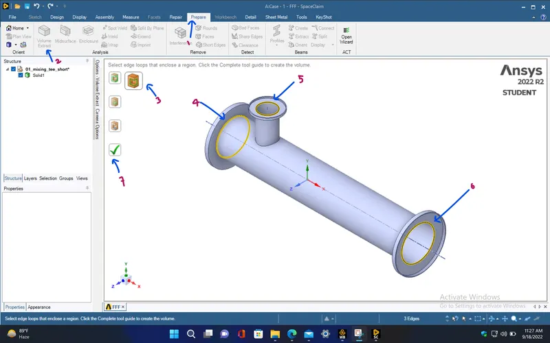
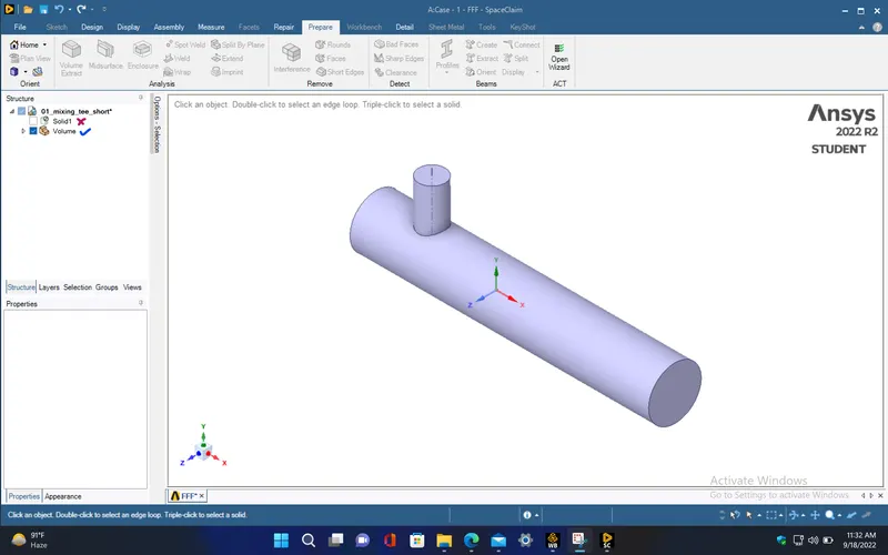
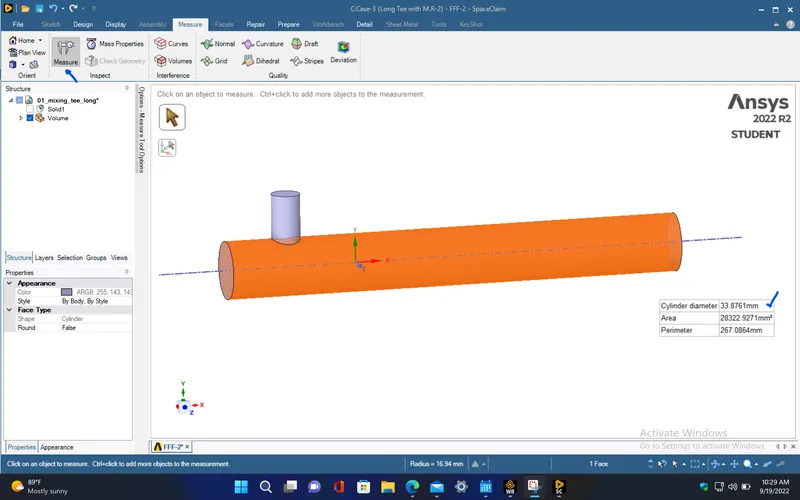
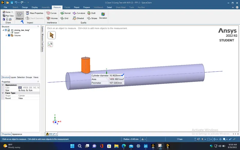
- Measure the dimensions of the model since it will be required for finding out the analytical results.
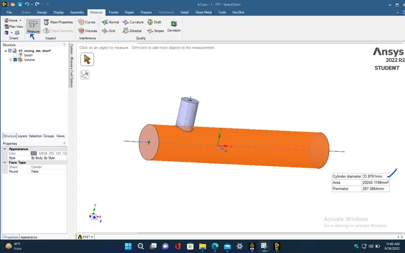
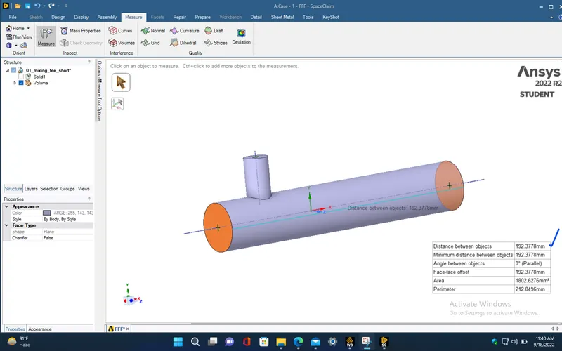
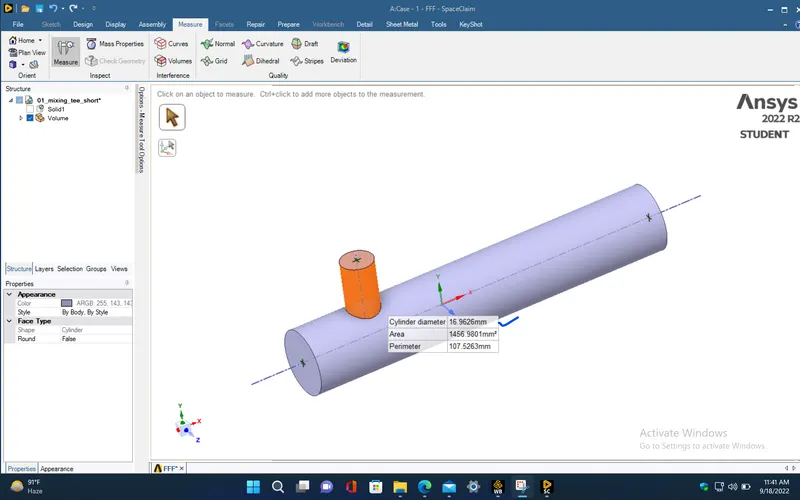
- Now, close spaceclaim window and open mesh window from the Ansys workbench and create named selections by giving required name for every fluid surfaces.
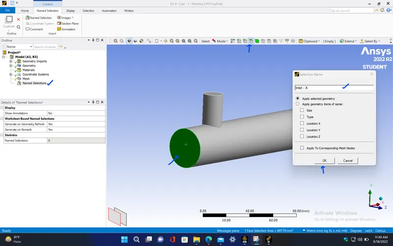
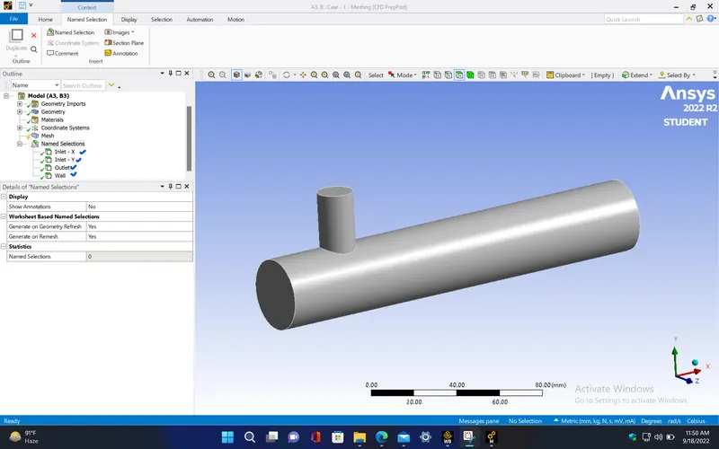
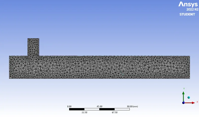
- Generate mesh for the domain by giving the mesh element size as 3mm.
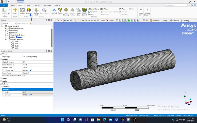
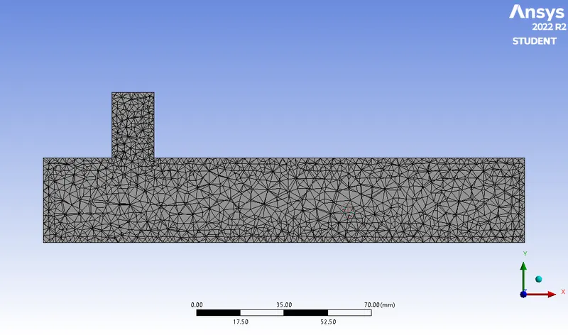
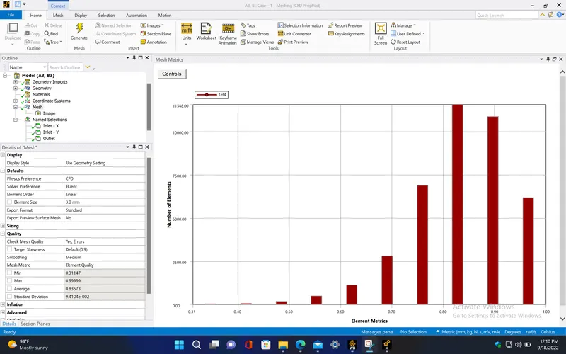
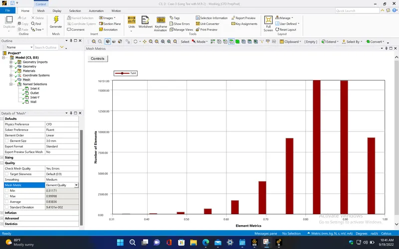
- Check the element quality criteria for the generated mesh.
SOLVING :
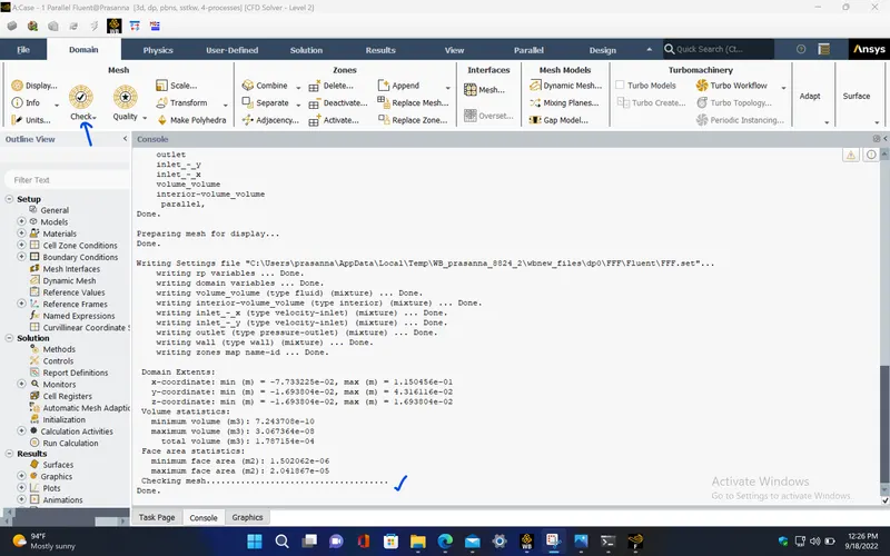
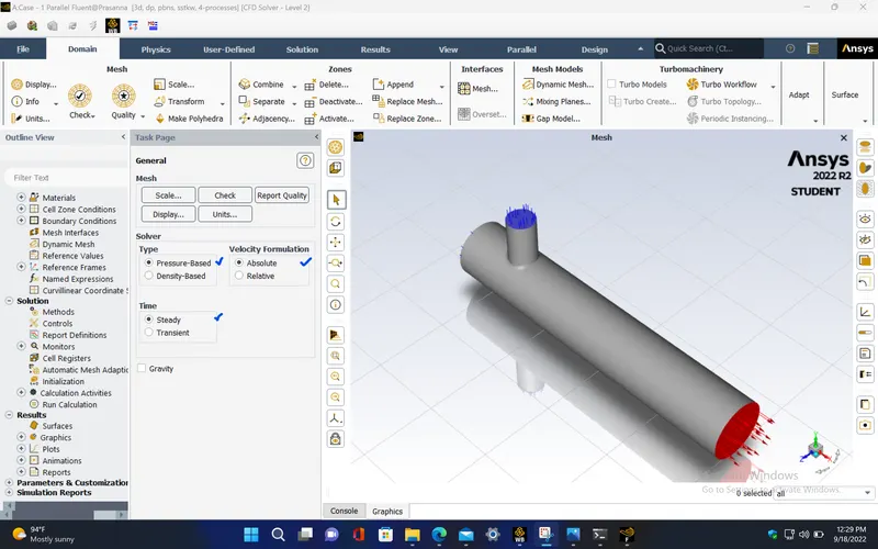
- After meshing, close the mesh window and open setup window from workbench. Here, perform the quality check for before setting up the domain.
|
Cells |
Faces |
Nodes |
|
40003 |
83255 |
8385 |
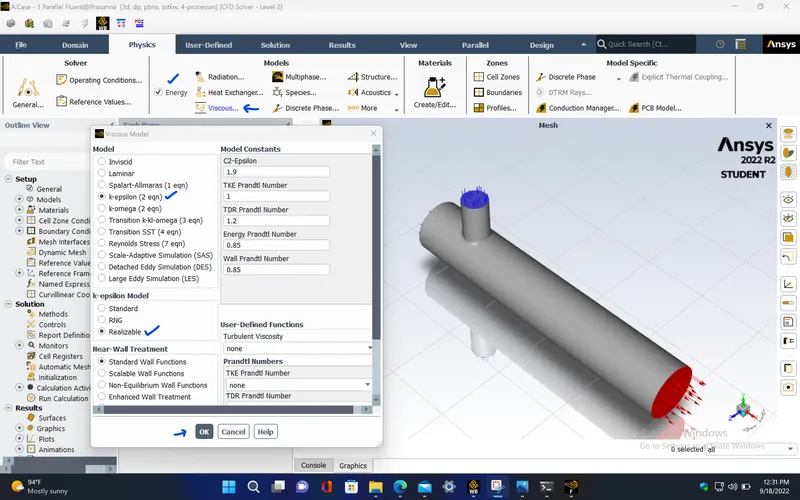
- Now, setup the domain with required boundary conditions and solver type needed for this case study,
|
Model |
Settings |
|
Space |
3D |
|
Time |
Steady |
|
Viscous |
Realizable k-epsilon turbulence model |
|
Wall Treatment |
Standard Wall Functions |
|
Heat Transfer |
Enabled |
MATERIAL PROPERTIES :
|
Fluid |
air |
|
Density |
1.225 kg/m^3 |
|
Cp (Specific Heat) |
1006.43 J/(kg K) |
|
Thermal Conductivity |
0.0242 W/(m K) |
|
Viscosity |
1.7894e-05 kg/(m s) |
|
Molecular Weight |
28.966 kg/kmol |
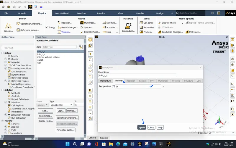
BOUNDARY CONDITIONS :
|
inlet_-_x |
|
|
Velocity Specification Method |
Magnitude, Normal to Boundary |
|
Reference Frame |
Absolute |
|
Velocity Magnitude [m/s] |
3 |
|
Temperature [C] |
36 |
|
inlet_-_y |
|
|
Velocity Specification Method |
Magnitude, Normal to Boundary |
|
Reference Frame |
Absolute |
|
Velocity Magnitude [m/s] |
6 |
|
Temperature [C] |
19 |
|
outlet |
|
|
Backflow Reference Frame |
Absolute |
|
Gauge Pressure [Pa] |
0 |
|
Pressure Profile Multiplier |
1 |
|
Backflow Total Temperature [C] |
26.85 |
|
Backflow Direction Specification Method |
Normal to Boundary |
|
Backflow Pressure Specification |
Total Pressure |
|
wall |
|
|
Wall Motion |
Stationary Wall |
|
Shear Boundary Condition |
No Slip |





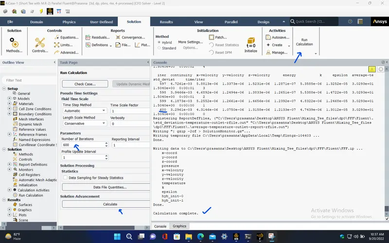
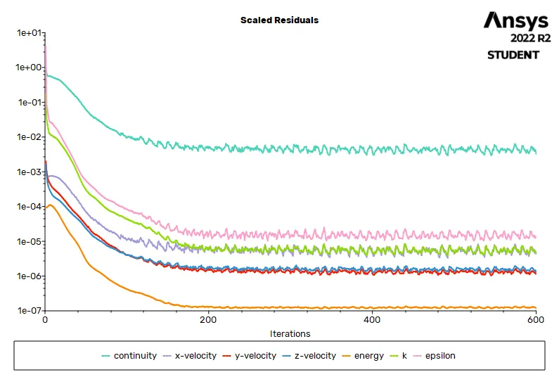
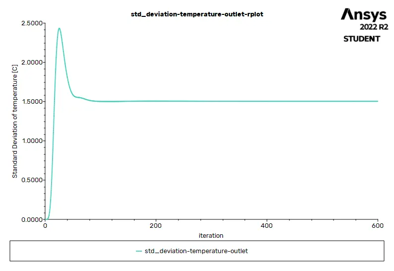
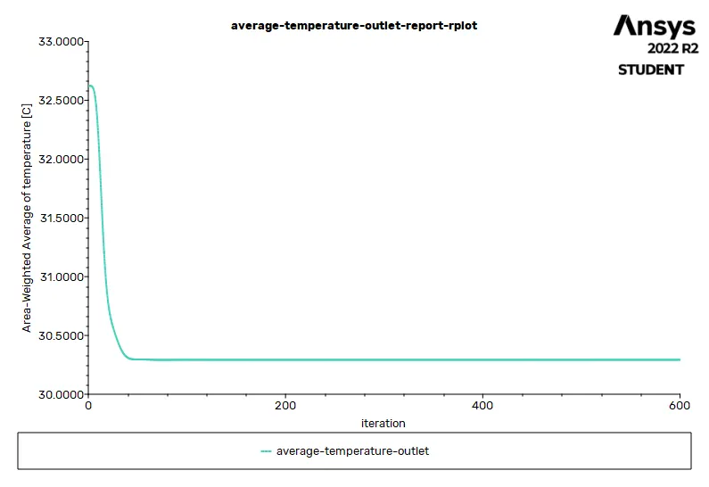
- Now, run the simulation for 600 iterations. This is more than enough for this model to get a converged solution for the average temperature at outlet.
RESIDUALS PLOT :
STANDARD DEVIATION PLOT FOR TEMPERATURE AT OUTLET :
AVERAGE TEMPERATURE AT OUTLET PLOT :
Average temperature at outlet :
Average velocity at outlet:

SOLUTION STATUS :
Total number of iterations : 600
|
Value |
Absolute Criteria |
Convergence Status |
|
|
continuity |
0.003296109 |
0.001 |
Not Converged |
|
x-velocity |
4.314571e-06 |
0.001 |
Converged |
|
y-velocity |
1.075011e-06 |
0.001 |
Converged |
|
z-velocity |
1.31578e-06 |
0.001 |
Converged |
|
energy |
1.213329e-07 |
1e-06 |
Converged |
|
k |
4.743911e-06 |
0.001 |
Converged |
|
epsilon |
1.301214e-05 |
0.001 |
Converged |
REPORT DEFINITIONS :
|
average-temperature-outlet |
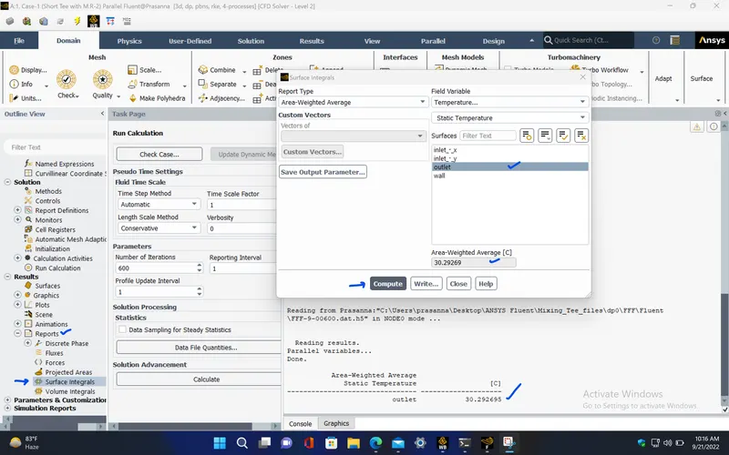
30.29269 |
C |
|
std_deviation-temperature-outlet |
1.503951 |
C |
POST PROCESSING :
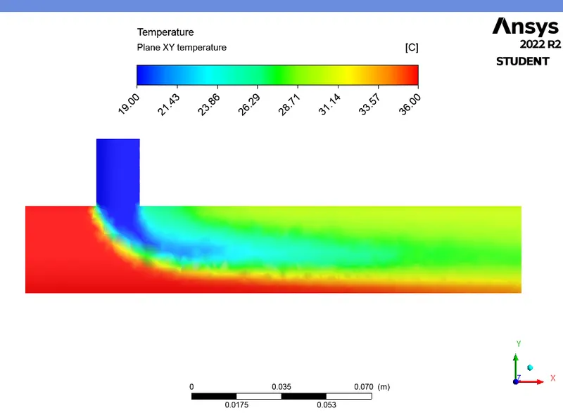
TEMPERATURE CONTOUR PLOT :
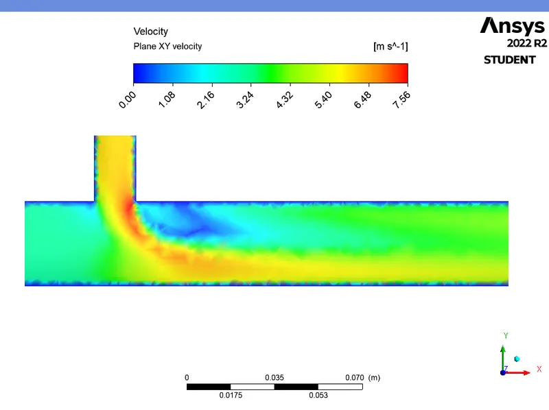
VELOCITY CONTOUR PLOT :
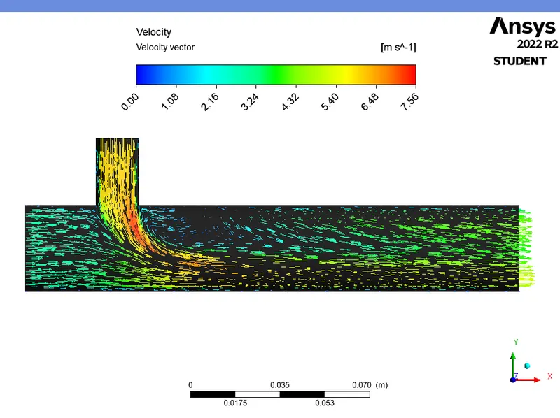
VELOCITY VECTOR PLOT :
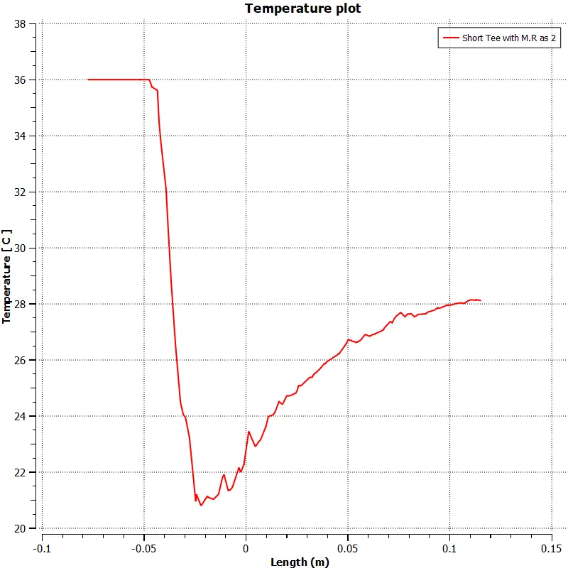
Plot for the temperature at the centre over the x- axis length of the model :
Plot for the velocity at the centre over the x- axis length of the model :
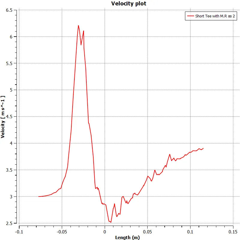
2. Short Tee with M.R - 4 (k-epsilon) :
- Similarly, repeat the same procedure for this case and the only change to be done is , the cold air inlet velocity is changed to 12 m/s.
|
Model |
Settings |
|
Space |
3D |
|
Time |
Steady |
|
Viscous |
Realizable k-epsilon turbulence model |
|
Wall Treatment |
Standard Wall Functions |
|
Heat Transfer |
Enabled |
MATERIAL PROPERTIES :
|
Fluid |
air |
|
Density |
1.225 kg/m^3 |
|
Cp (Specific Heat) |
1006.43 J/(kg K) |
|
Thermal Conductivity |
0.0242 W/(m K) |
|
Viscosity |
1.7894e-05 kg/(m s) |
|
Molecular Weight |
28.966 kg/kmol |
BOUNDARY CONDITIONS :
|
inlet_-_x |
|
|
Velocity Specification Method |
Magnitude, Normal to Boundary |
|
Reference Frame |
Absolute |
|
Velocity Magnitude [m/s] |
3 |
|
Supersonic/Initial Gauge Pressure [Pa] |
0 |
|
Temperature [C] |
36 |
|
inlet_-_y |
|
|
Velocity Specification Method |
Magnitude, Normal to Boundary |
|
Reference Frame |
Absolute |
|
Velocity Magnitude [m/s] |
12 |
|
Supersonic/Initial Gauge Pressure [Pa] |
0 |
|
Temperature [C] |
19 |
|
outlet |
|
|
Backflow Reference Frame |
Absolute |
|
Gauge Pressure [Pa] |
0 |
|
wall |
|
|
Wall Motion |
Stationary Wall |
|
Shear Boundary Condition |
No Slip |
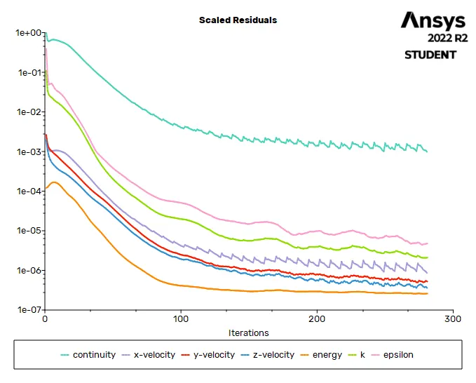
RESIDUALS PLOT :
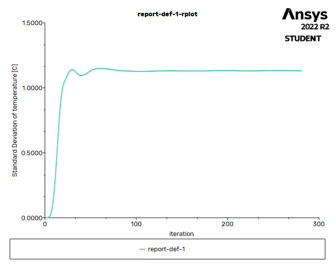
STANDARD DEVIATION PLOT FOR TEMPERATURE AT OUTLET :
AVERAGE TEMPERATURE AT OUTLET PLOT :
Average temperature at outlet :
Average velocity at outlet:
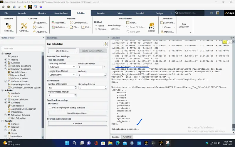
SOLUTION STATUS :
Total number of iterations : 297
|
Value |
Absolute Criteria |
Convergence Status |
|
|
continuity |
0.0009684185 |
0.001 |
Converged |
|
x-velocity |
8.114843e-07 |
0.001 |
Converged |
|
y-velocity |
4.776282e-07 |
0.001 |
Converged |
|
z-velocity |
3.399351e-07 |
0.001 |
Converged |
|
energy |
2.546249e-07 |
1e-06 |
Converged |
|
k |
1.766033e-06 |
0.001 |
Converged |
|
epsilon |
3.711411e-06 |
0.001 |
Converged |
REPORT DEFINITIONS :
|
average-temperature-outlet |
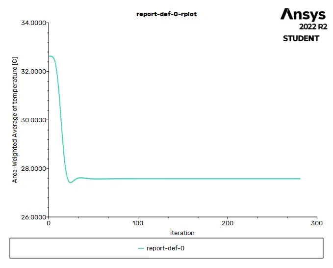
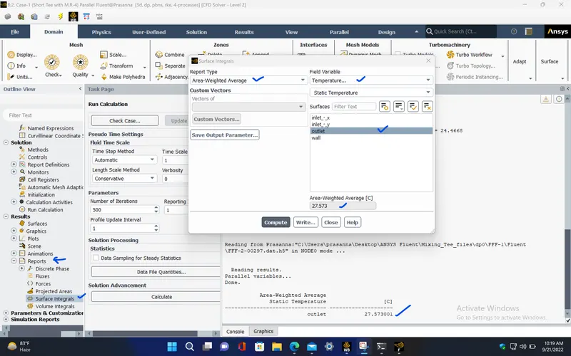
27.573 |
C |
|
std-deviation-temperature-outlet |
1.132525 |
C |
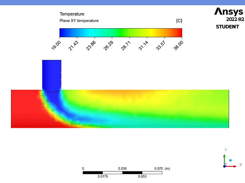
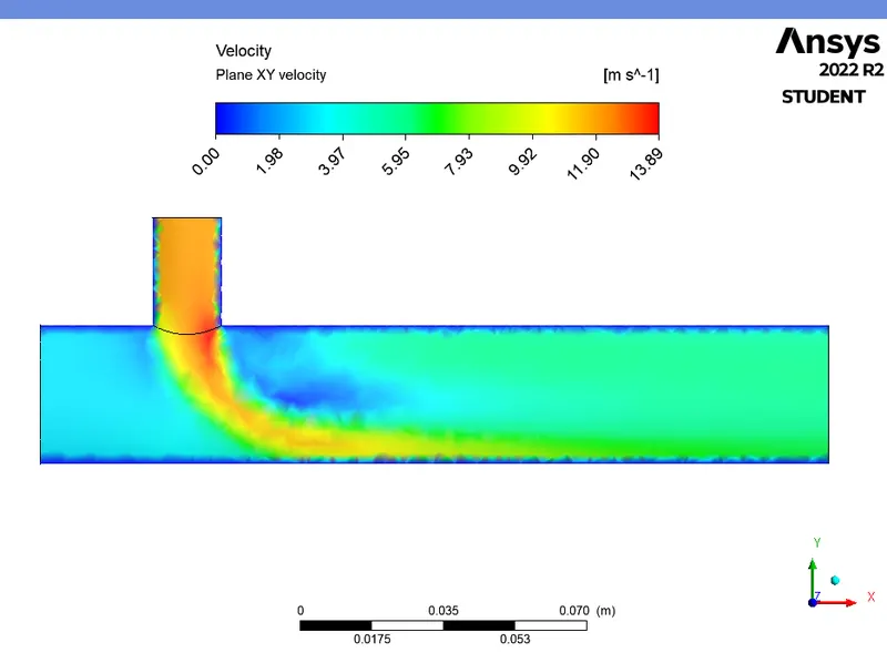
TEMPERATURE CONTOUR PLOT :
VELOCITY CONTOUR PLOT :
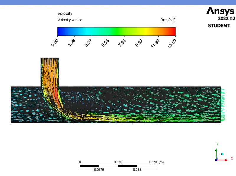
VELOCITY VECTOR PLOT :
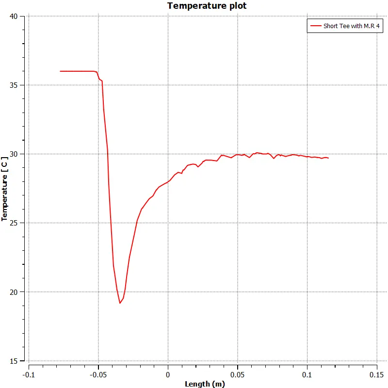
Plot for the temperature at the centre over the x- axis length of the model :
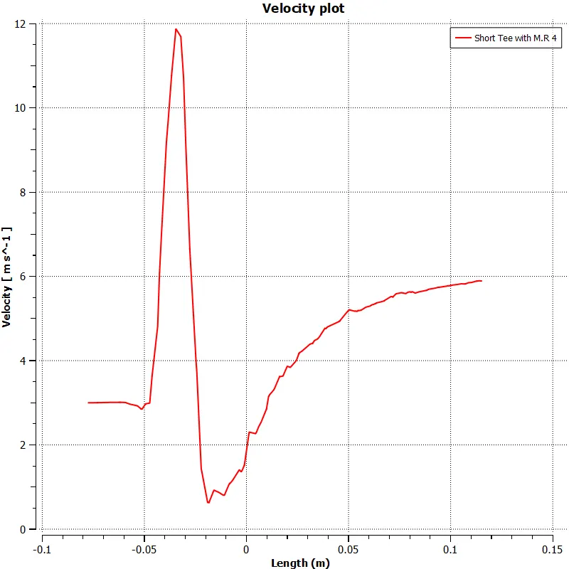
Plot for the velocity at the centre over the x- axis length of the model :
3. Short Tee with M.R - 4 and choosing the k-omega SST turbulence model type :
|
Model |
Settings |
|
Space |
3D |
|
Time |
Steady |
|
Viscous |
SST k-omega turbulence model |
|
Heat Transfer |
Enabled |
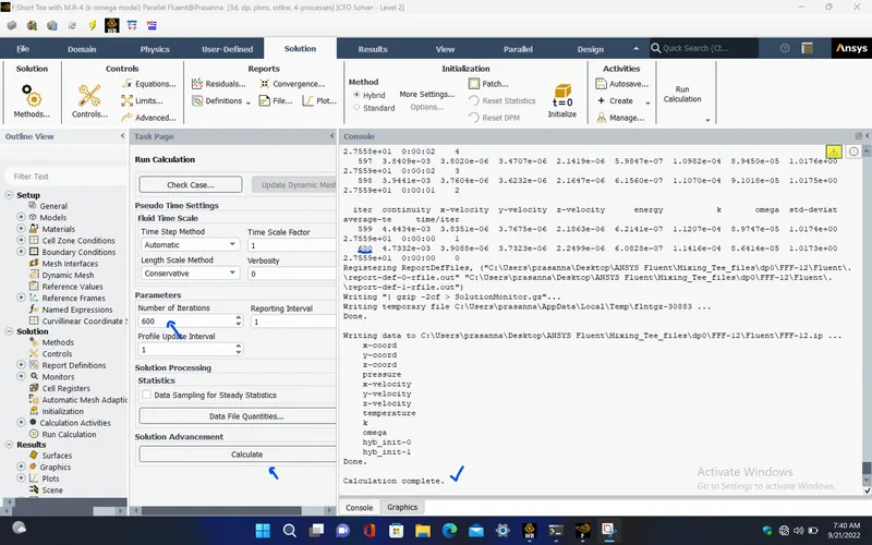
RESIDUALS PLOT :
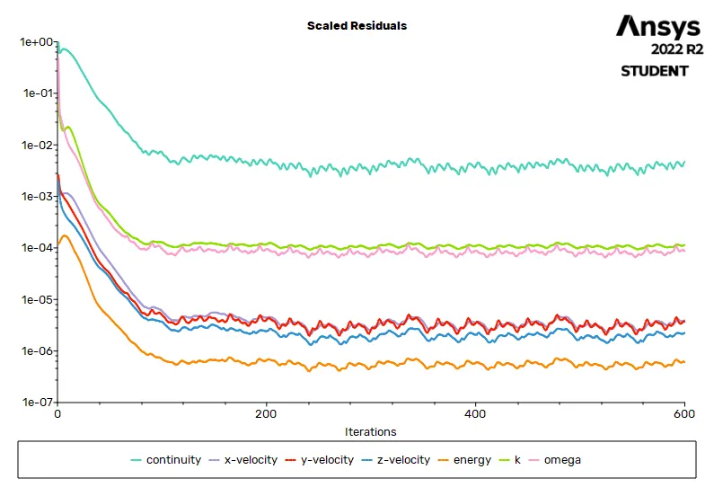
STANDARD DEVIATION PLOT FOR TEMPERATURE AT OUTLET :
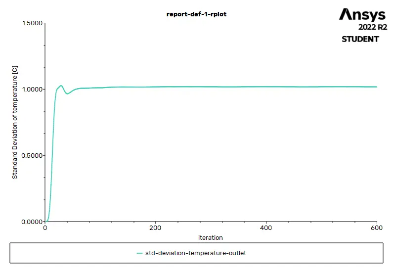
AVERAGE TEMPERATURE AT OUTLET PLOT :
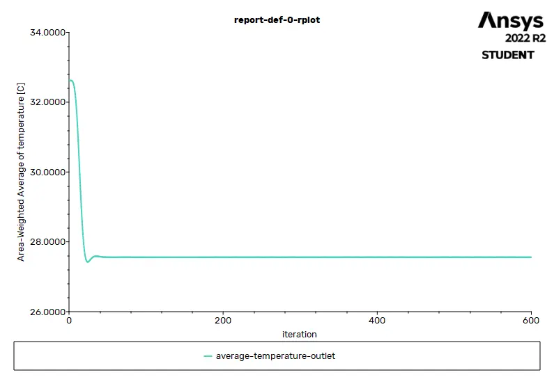
SOLUTION STATUS :
Total number of iterations : 600
|
Value |
Absolute Criteria |
Convergence Status |
|
|
continuity |
0.004733204 |
0.001 |
Not Converged |
|
x-velocity |
3.908848e-06 |
0.001 |
Converged |
|
y-velocity |
3.732335e-06 |
0.001 |
Converged |
|
z-velocity |
2.249888e-06 |
0.001 |
Converged |
|
energy |
6.082842e-07 |
1e-06 |
Converged |
|
k |
0.0001141626 |
0.001 |
Converged |
|
omega |
8.641424e-05 |
0.001 |
Converged |
REPORT DEFINITIONS :
|
std-deviation-temperature-outlet |
1.01731 |
C |
|
average-temperature-outlet |
27.55882 |
C |
- If we compare previous two cases involving k-epsilon and k-omega SST, solution is converged at 297th iteration for k-epsilon case whereas, in k-omega , it is not getting converged till 600th iteration.
- Hence, k-epsilon is choosen over k-omega SST for the remaining cases.
4. Case - 2 - Long Tee with M.R - 2 :
PRE-PROCESSING :
- Now, import the long tee model into spaceclaim window. This long mixing tee model is larger in length compared to the short tee model but the diameter in both fluid stream inlets are same as previous case. This larger length can help in increasing the temperature distribution over the domain compared to the short tee model.
- Repeat the same procedure as done in previous cases.
|
Cells |
Faces |
Nodes |
|
57101 |
118537 |
11798 |
SOLVING :
|
Model |
Settings |
|
Space |
3D |
|
Time |
Steady |
|
Viscous |
Realizable k-epsilon turbulence model |
|
Wall Treatment |
Standard Wall Functions |
|
Heat Transfer |
Enabled |
MATERIAL PROPERTIES :
|
Fluid |
air |
|
Density |
1.225 kg/m^3 |
|
Cp (Specific Heat) |
1006.43 J/(kg K) |
|
Thermal Conductivity |
0.0242 W/(m K) |
|
Viscosity |
1.7894e-05 kg/(m s) |
|
Molecular Weight |
28.966 kg/kmol |
BOUNDARY CONDITIONS :
|
inlet-x |
|
|
Velocity Specification Method |
Magnitude, Normal to Boundary |
|
Reference Frame |
Absolute |
|
Velocity Magnitude [m/s] |
3 |
|
Supersonic/Initial Gauge Pressure [Pa] |
0 |
|
Temperature [C] |
36 |
|
inlet-y |
|
|
Velocity Specification Method |
Magnitude, Normal to Boundary |
|
Reference Frame |
Absolute |
|
Velocity Magnitude [m/s] |
6 |
|
Supersonic/Initial Gauge Pressure [Pa] |
0 |
|
Temperature [C] |
19 |
|
outlet |
|
|
Backflow Reference Frame |
Absolute |
|
Gauge Pressure [Pa] |
0 |
|
Backflow Direction Specification Method |
Normal to Boundary |
|
wall |
|
|
Wall Motion |
Stationary Wall |
|
Shear Boundary Condition |
No Slip |
- Run the simulations for 500 iterations.
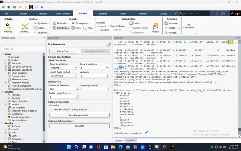
RESIDUALS PLOT :
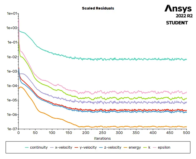
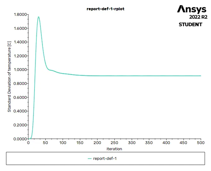
STANDARD DEVIATION PLOT FOR TEMPERATURE AT OUTLET :
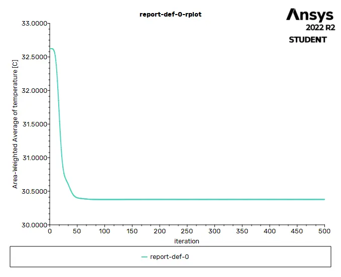
AVERAGE TEMPERATURE AT OUTLET PLOT :
Average temperature at outlet :

Average velocity at outlet:

SOLUTION STATUS :
Total number of iterations : 500
|
Value |
Absolute Criteria |
Convergence Status |
|
|
continuity |
0.005662669 |
0.001 |
Not Converged |
|
x-velocity |
6.107166e-06 |
0.001 |
Converged |
|
y-velocity |
1.888871e-06 |
0.001 |
Converged |
|
z-velocity |
1.4452e-06 |
0.001 |
Converged |
|
energy |
1.407584e-07 |
1e-06 |
Converged |
|
k |
1.279795e-05 |
0.001 |
Converged |
|
epsilon |
3.19655e-05 |
0.001 |
Converged |
REPORT DEFINITIONS :
|
average-temperature-outlet |
30.37805 |
C |
|
std-deviation-temperature-outlet |
0.9109911 |
C |
POST PROCESSING :
TEMPERATURE CONTOUR PLOT :
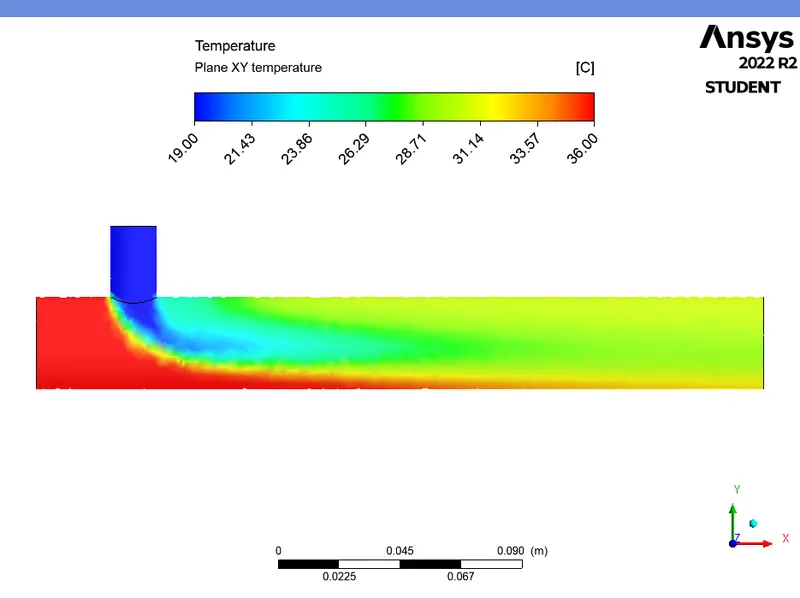
VELOCITY CONTOUR PLOT :
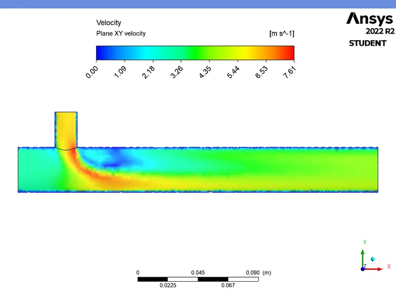
VELOCITY VECTOR PLOT :
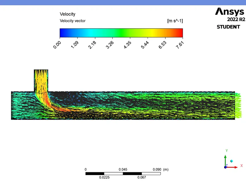
Plot for the temperature at the centre over the x- axis length of the model :
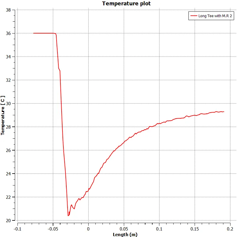
Plot for the velocity at the centre over the x- axis length of the model :
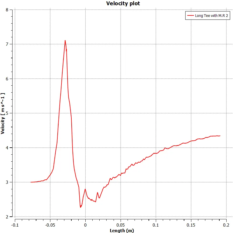
5. Long Tee with M.R - 4 :
- In this case, just change the inlet-y velocity to 12 m/s in the boundary conditions.
|
Cells |
Faces |
Nodes |
|
57101 |
118537 |
11798 |
|
Model |
Settings |
|
Space |
3D |
|
Time |
Steady |
|
Viscous |
Realizable k-epsilon turbulence model |
|
Wall Treatment |
Standard Wall Functions |
|
Heat Transfer |
Enabled |
MATERIAL PROPERTIES :
|
Fluid |
air |
|
Density |
1.225 kg/m^3 |
|
Cp (Specific Heat) |
1006.43 J/(kg K) |
|
Thermal Conductivity |
0.0242 W/(m K) |
|
Viscosity |
1.7894e-05 kg/(m s) |
|
Molecular Weight |
28.966 kg/kmol |
BOUNDARY CONDITIONS :
|
inlet-x |
|
|
Velocity Specification Method |
Magnitude, Normal to Boundary |
|
Reference Frame |
Absolute |
|
Velocity Magnitude [m/s] |
3 |
|
Supersonic/Initial Gauge Pressure [Pa] |
0 |
|
Temperature [C] |
36 |
|
inlet-y |
|
|
Velocity Specification Method |
Magnitude, Normal to Boundary |
|
Reference Frame |
Absolute |
|
Velocity Magnitude [m/s] |
12 |
|
Supersonic/Initial Gauge Pressure [Pa] |
0 |
|
Temperature [C] |
19 |
|
outlet |
|
|
Backflow Reference Frame |
Absolute |
|
Gauge Pressure [Pa] |
0 |
|
Backflow Direction Specification Method |
Normal to Boundary |
|
wall |
|
|
Wall Motion |
Stationary Wall |
|
Shear Boundary Condition |
No Slip |
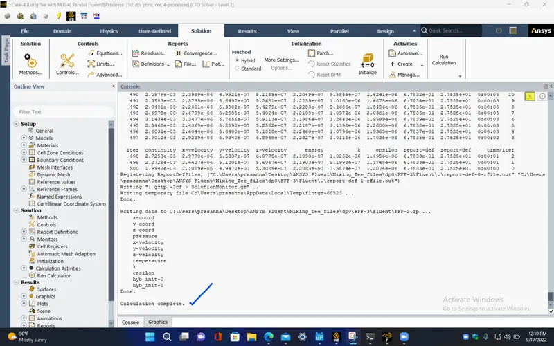
- Run the simulation for 500 iterations
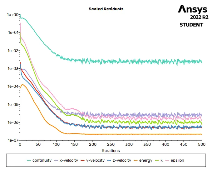
RESIDUALS PLOT :
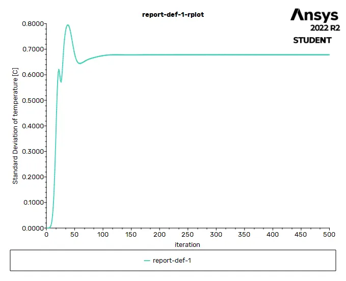
STANDARD DEVIATION PLOT FOR TEMPERATURE AT OUTLET :
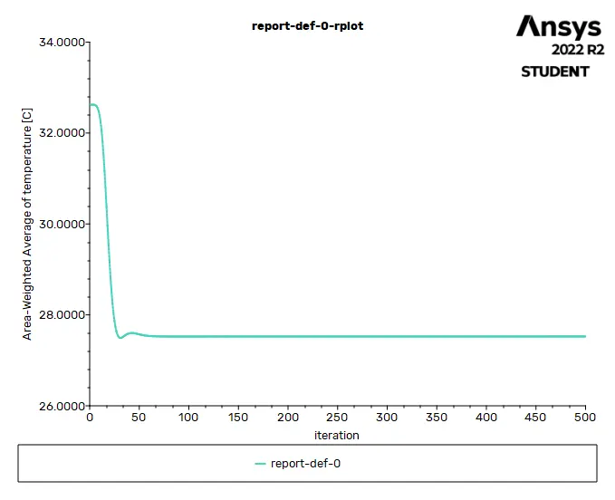
AVERAGE TEMPERATURE AT OUTLET PLOT :
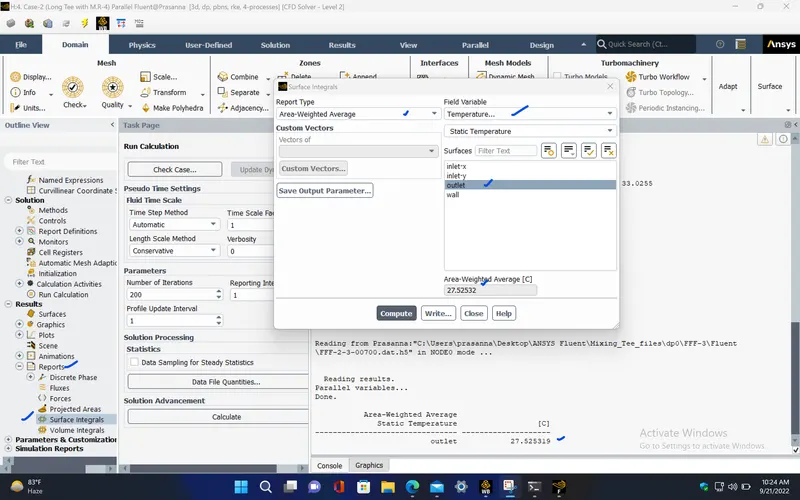
Average temperature at outlet :
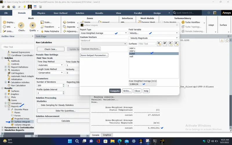
Average velocity at outlet:
SOLUTION STATUS :
Total number of iterations : 500
|
Value |
Absolute Criteria |
Convergence Status |
|
|
continuity |
0.001946774 |
0.001 |
Not Converged |
|
x-velocity |
2.137609e-06 |
0.001 |
Converged |
|
y-velocity |
4.766194e-07 |
0.001 |
Converged |
|
z-velocity |
4.73691e-07 |
0.001 |
Converged |
|
energy |
2.24108e-07 |
1e-06 |
Converged |
|
k |
8.153712e-07 |
0.001 |
Converged |
|
epsilon |
1.433163e-06 |
0.001 |
Converged |
REPORT DEFINITIONS :
|
average-temperature-outlet |
27.52532 |
C |
|
std-deviation-outlet |
0.6782932 |
C |
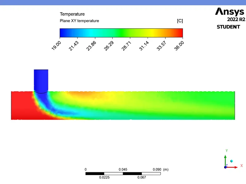
TEMPERATURE CONTOUR PLOT :
VELOCITY CONTOUR PLOT :
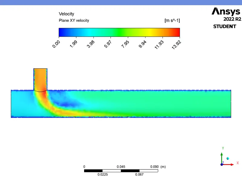
VELOCITY VECTOR PLOT :
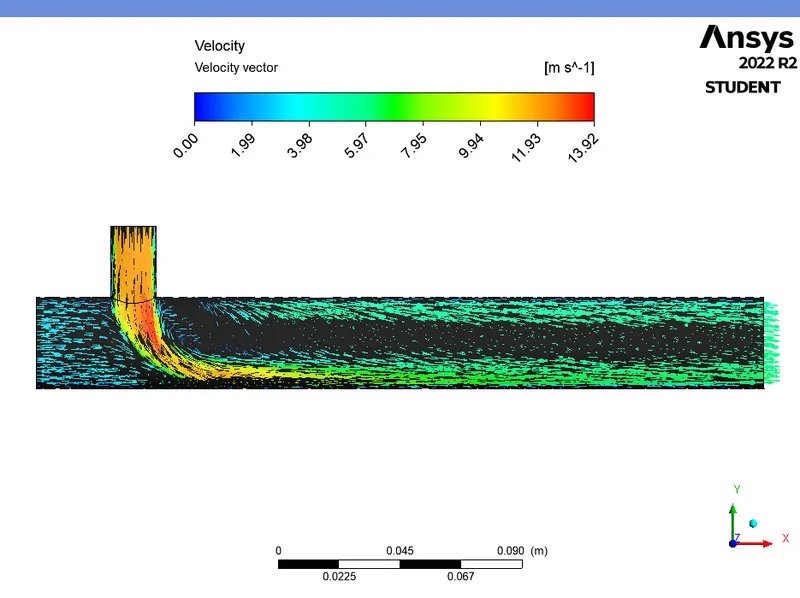
Plot for the temperature at the centre over the x- axis length of the model :
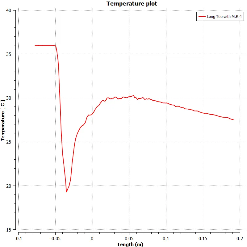
Plot for the velocity at the centre over the x- axis length of the model :
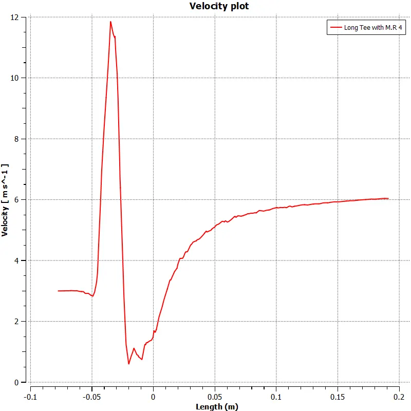
MESH INDEPENDENT STUDY :
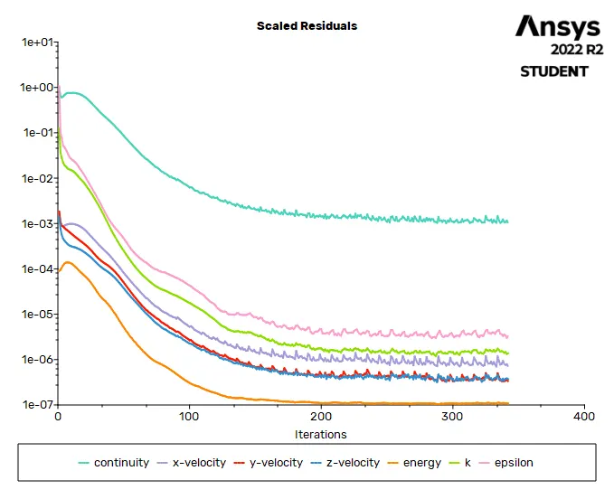
6. Short Tee with M.R - 4 (2mm mesh length):
- In the previous cases, we have used 3mm as the mesh length. In this case, we are changing the mesh length to 2mm while keeping all other parameters same as in Short Tee with M.R - 4 case.
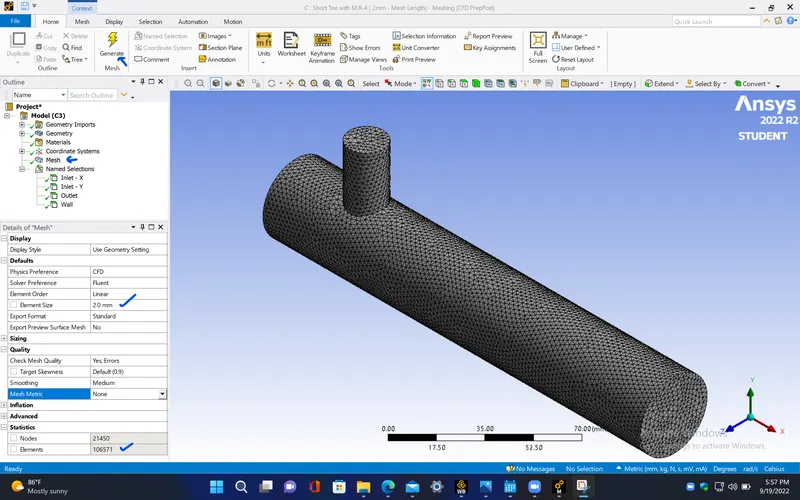
- Here, for 2mm mesh length, the total number of mesh elements increased to 106571 whereas in previous case, it was 40003 elements for 3mm mesh length for short tee model.
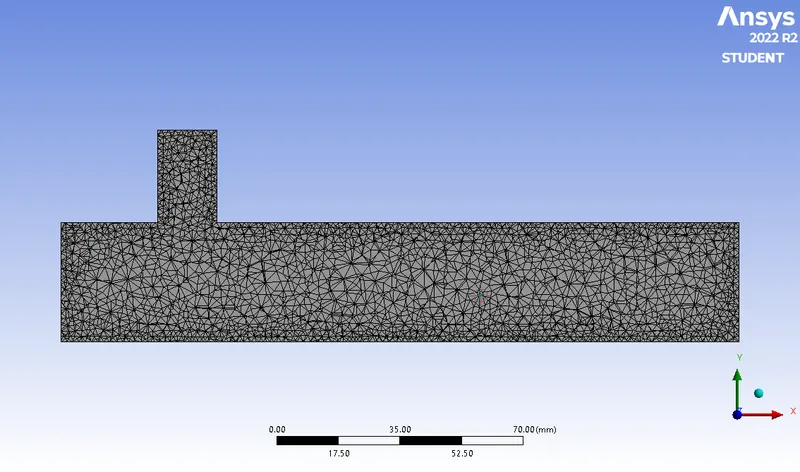
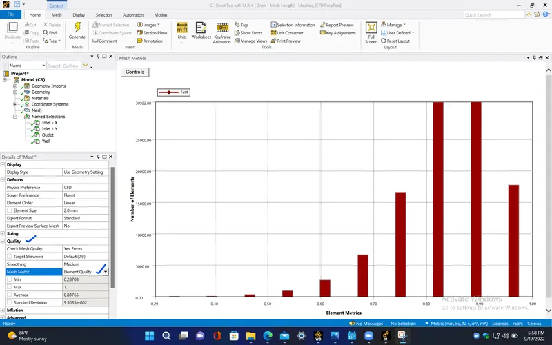
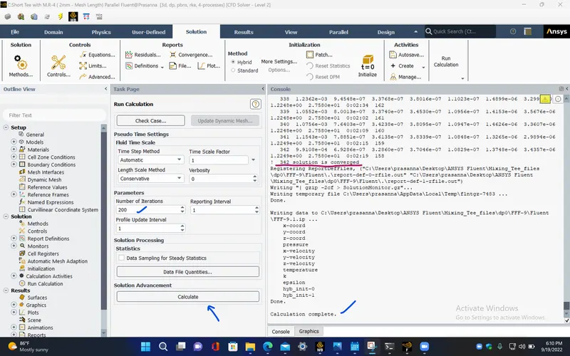
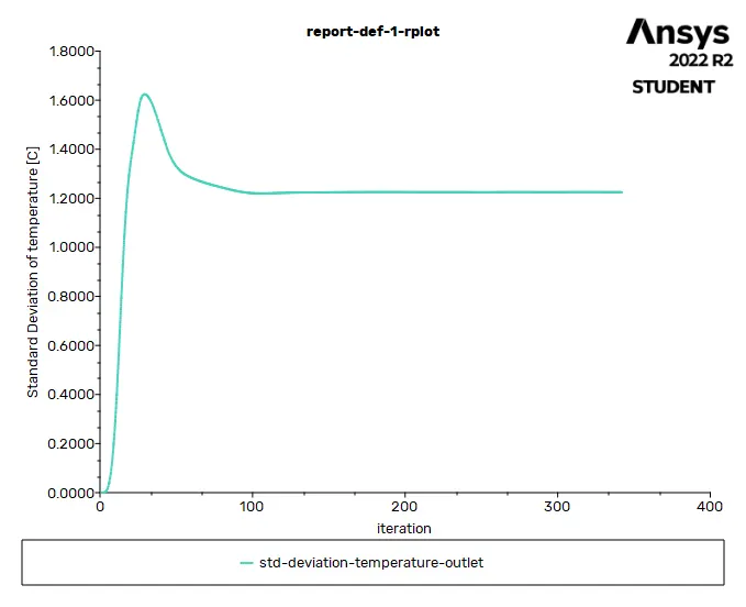
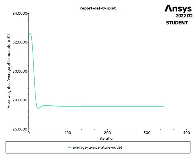
- After simulation, we can observe that the solution gets converged at 342th iteration whereas, for 3mm mesh length, the solution is coverged at 297th iteration.
- Therefore, it takes more iterations and also the computational time for simulating the same short tee model compared to the previous case, but the accuracy of the temperature at outlet is increased in this case, since it has more number of elements.
RESIDUALS PLOT :
STANDARD DEVIATION PLOT FOR TEMPERATURE AT OUTLET :
AVERAGE TEMPERATURE AT OUTLET PLOT :
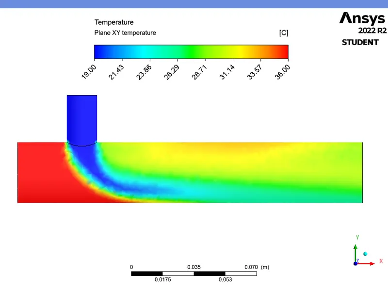
- In the below contour plot, we can observe that the region where the two fluid streams mixing together has less distortion in temperature distribution compared to the one that has 3mm mesh length contour plot.
TEMPERATURE CONTOUR PLOT :
7. Short Tee with M.R - 4 (5mm mesh length) :
- In this case, we use 5mm mesh length for the short tee model while keeping all other parameters unchanged as in the previous case.
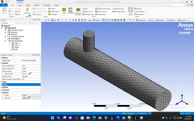
- Here, number of mesh elements is decreased to 14248.
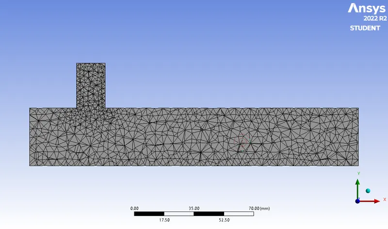
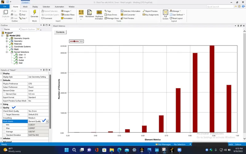
- After setting up the domain, run the simlation for 300 number of iterations.
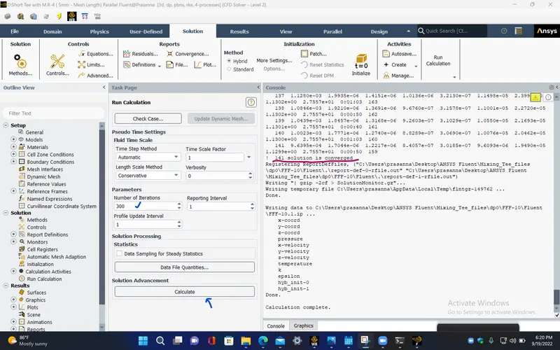
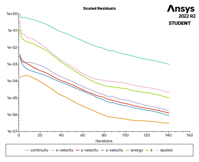
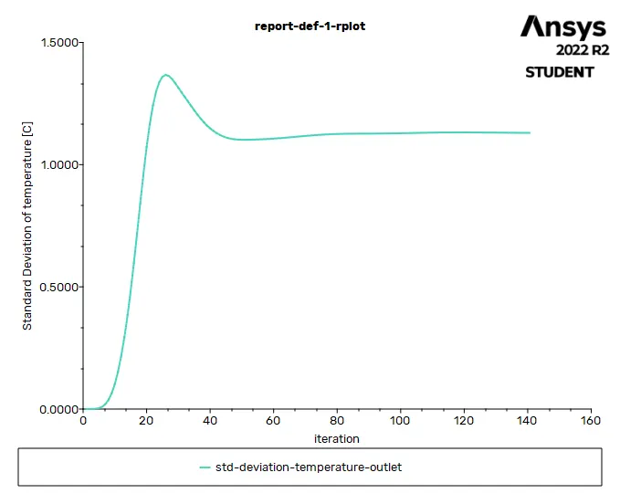
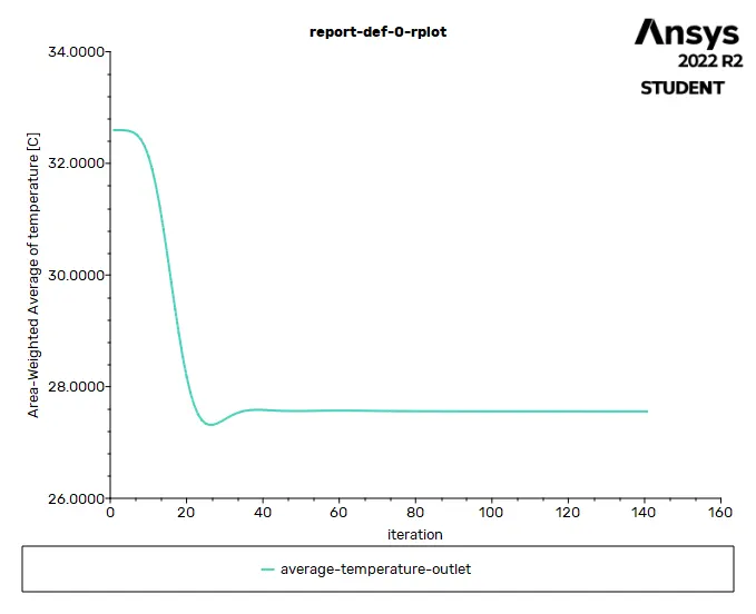
- Here, The solution got converged at 141th iteration of the simultion which is less compared to the previous case.
RESIDUALS PLOT :
STANDARD DEVIATION PLOT FOR TEMPERATURE AT OUTLET :
AVERAGE TEMPERATURE AT OUTLET PLOT :
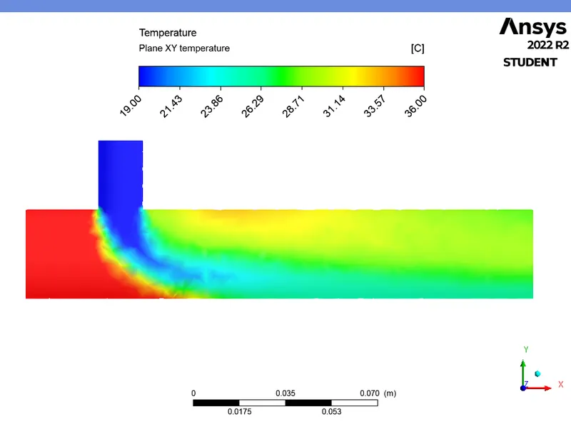
- Here, the distortion in mixing region is more compared to the previous case since it has the larger mesh length compared to others.
TEMPERATURE CONTOUR PLOT :
RESULTS :
Google drive link :
https://drive.google.com/file/d/1wrD2oNpDJRoXLTj7zgGQx5VBGLOAv-Rw/view?usp=sharing
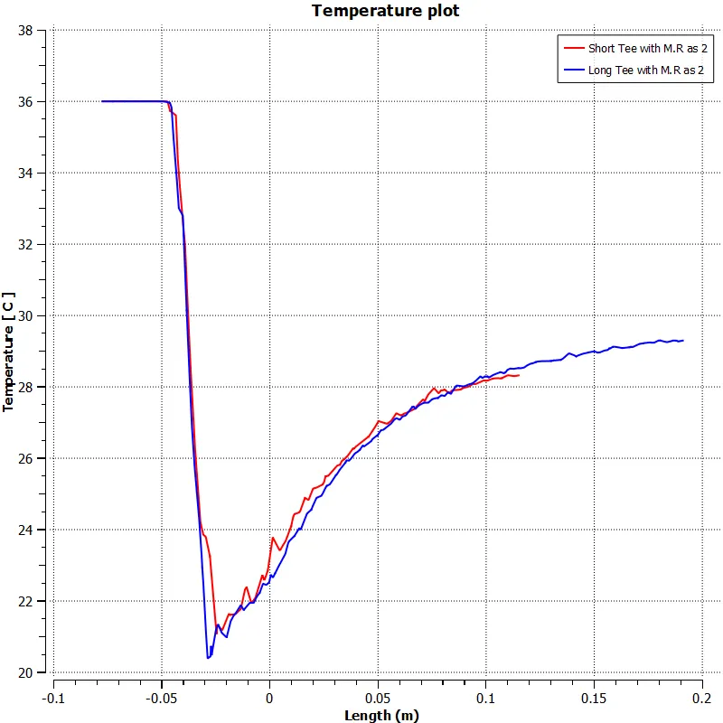
1. Temperature comparison plot for short and long tee with M.R of 2,
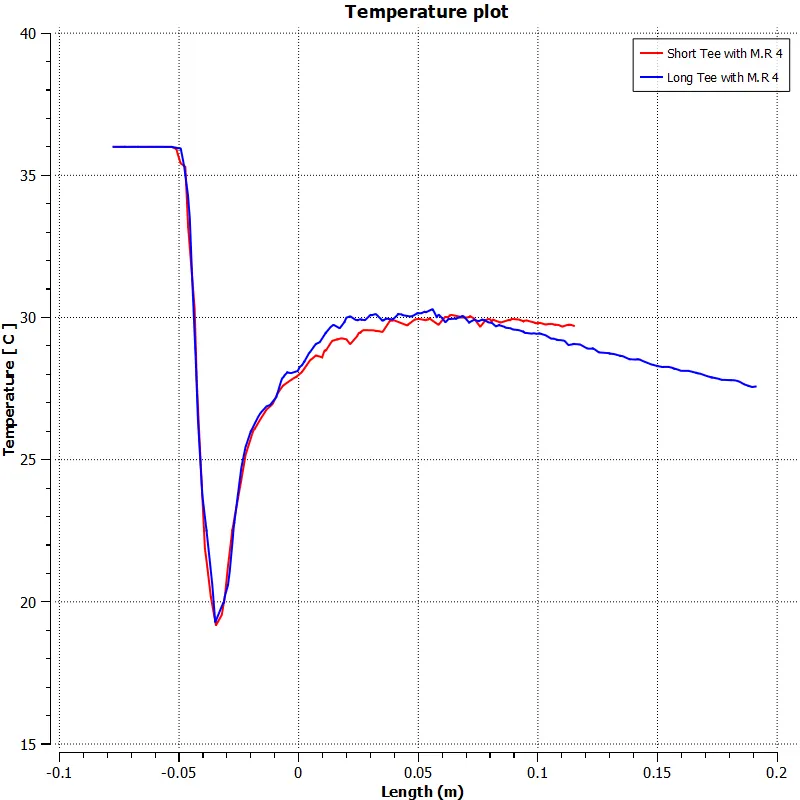
2. Temperature comparison plot for short and long tee with M.R of 4,
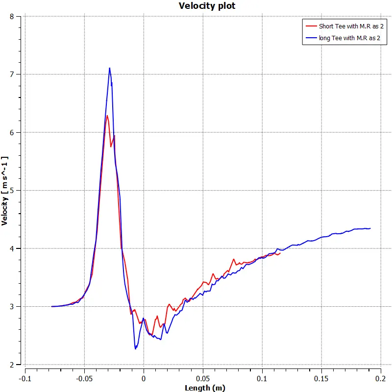
3. Velocity comparison plot for short and long tee model with M.R of 2,
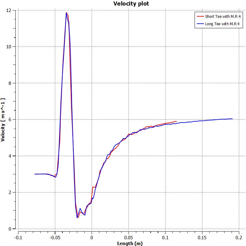
4. Velocity comparison plot for short and long tee model with M.R of 4,
CONCLUSION :
After finding out the simulation results for all the cases, we can compare and validate the results by using analytical solution,
|
Mixing Tee models |
Momentum ratios |
Tuurbulence model |
Mesh element length(mm) |
Number of mesh elements |
Average Temperature at outlet (in ‘C’) |
Error (in %) |
Average Velocity at outlet (in ‘m/s’) |
Error (in %) |
||
|
Final solution |
Analytical solution |
Final solution |
Analytical solution
|
|||||||
|
Short Tee |
Momentum ratio = 2 |
K-epsilon |
3 |
40003 |
30.29269 |
30.32238 |
0.098 |
4.492601 |
4.50435 |
0.26 |
|
Momentum ratio = 4 |
k-epsilon |
2 |
106571 |
27.579587 |
27.487689 |
0.33 |
6.0307311 |
6.0087 |
0.3666 |
|
|
3 |
40003 |
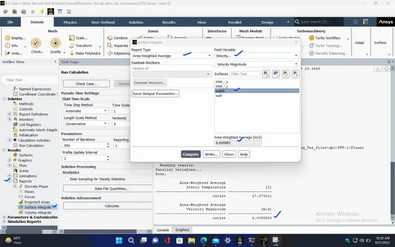
27.573 |
0.31 |
6.00998 |
0.02 |
|||||
|
5 |
14248 |
27.556686 |
0.25 |
6.0251548 |
0.2738 |
|||||
|
k–omega SST |
3 |
40003 |
27.558817 |
0.258 |
6.0339689 |
0.42 |
||||
|
Long Tee |
Momentum ratio = 2 |
k-epsilon |
3 |
57101 |
30.37805 |
30.32238 |
0.18 |
4.4899 |
4.50435 |
0.32 |
|
Momentum ratio = 4 |
k-epsilon |
3 |
57101 |
27.52532 |
27.487689 |
0.137 |
5.9941341 |
6.0087 |
0.2424 |
|
From the above table, we can conclude that the mixing effectiveness is greater in long tee model with momentum ratio of 4, since the extra length of the model cause the temperature of the air streams to diffuse more compared to other cases and also increase in the cold air inlet velocity increases the effectiveness of mixing.