Week 4 - CHT Analysis on Exhaust port
AIM :
To simulate the flow of exhaust air with the velocity of 5 m/s at 700K through the given exhaust port model and perform the conjugate heat transfer analysis between the air and the exhaust port wall surface.
OBJECTIVES :
- To extract the volume for the fluid domain from the given eshaust port model in spaceclaim.
- To create inflation layers and different mesh element lengths for different cases and generate mesh.
- To setup and run the simulation.
- To post process the simulation results.
INTRODUCTION :
In this project, conjugate heat transfer analysis is to be performed in the given exhaust port model to find the convective heat transfer between the internal surface wall and the fluid (air) provided that the outer wall surface of the model has a heat transfer co-efficient of 20 W / m^2-K to the surrounding atmospheric air.
CHT Analysis and applications:
CHT means Conjugate Heat Transfer. It is the analysis done for finding heat transfer which occurs by means of both conduction( due to direct molecular interactions ) and convection( due to fluid bulk motion ).
It is a analysis of heat transfer between a solid and fluid domain by exchanging the thermal energy at the interface between them.
Typical applications of this analysis are the simulation of heat exchangers, cooling of electronic equipment, and general-purpose cooling and heating systems.
CASE SETUP :
- Consider the air is flowing through the inlets of the exhaust port at the velocity of 25 m/s at the temperature of 700K.
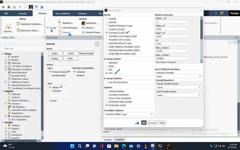
- In this analysis, our main focus is near the wall region of the exhaust port where the CHT occurs, so we choose K-omega SST turbulence model which will provide accurate results for near wall related analysis.
Here, we perform the mesh independency study to find out with mesh size gives more accurate simulation results with less computational time.
|
CASE STUDY |
MESH ELEMENT SIZE (in ‘mm’) |
|
|
Base mesh length |
Sizing |
|
|
CASE - 1 |
150 |
- |
|
CASE - 2 |
50 |
20 |
|
CASE - 3 |
25 |
15 |
Maintaining Y+ :
- It is an non-dimensional distance.
- It can be used to determine the first layer distance from the wall which is measured in terms of viscous length.
- Here, we have to maintain Y+ with respect to turbulence model.
- Since the turbulence model for this analysis is taken as K-omega SST, the Y+ value should be between 0 and 10.
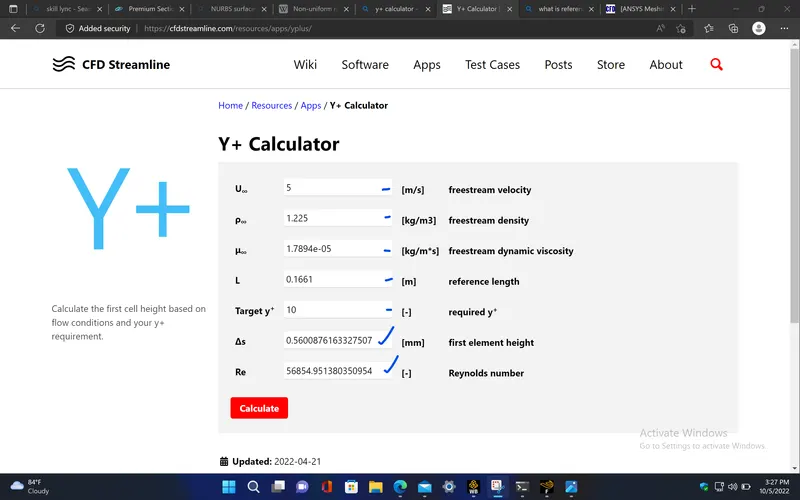
- Here, we take the Y+ value of 10 to calculate the first layer thickness.
Reynolds number :
It is a dimensionless number which is defined as the ratio of inertial force to the viscous force of the fluid.
`Re = rho * V * D / mu`
Where
- `rho = "Density of the fluid" ((kg)/m^3)`
- `V = "Velocity of the fluid"(m/s)`
- `mu ="Dynamic viscosity of the fluid" ((kg)/ (m.s))`
- `D = "Diameter of the fluid" (m)`
Prandtl number :
It is a dimensionless number which is defined as the ratio of momentum diffusivity to the thermal diffusivity of the fluid.
`Pr = nu / alpha`
Where,
- `nu ="kinematic viscosity of the fluid"(m^2 / s)`
- `alpha ="Thermal diffusivity"(m^2/s)`
Nusselt number :
It is a dimensionless number which is defined as the ratio of convective heat transfer to conductive heat transfer within the fluid region. It ranges between '0' and '1'. The value closer to '0' mean the heat transfer is mostly due to conduction ( due to direct molecular interactions ) and if the value is closer to '1', the heat transfer is mostly due to convection ( due to fluid bulk motion ).
Nusselt number (Nu) = Convective heat transfer / Conductive heat transfer
`Nu = h / ( k/D )`
`Nu = h * D / k`
Where,
- `h = "Heat transfer coefficient"(W/(m^2*K))`
- `k = "Thermal conductivity of the fluid/material"(W/(m*K))`
ANALYTICAL CALCULATION for verifying and validating HTC :
Here the properties of air is taken for the calculation purpose since the fluid which is flowing through the exhaust port is air,
- Density, `rho = 1.225 ((kg)/m^3)`
- Specific heat capacity, `C_p = 1006.43 (J/(kg.K))`
- Thermal conductivity, `k = 0.0242 (W/(m.K))`
- Dynamic viscosity, `mu = 1.7894*10^-5 ((kg)/(m.s))`
We know that Reynolds number,
`Re = rho * V * D / mu`
Where,
- Velocity, `V = 5 (m/s)`
- Diameter, `D = 0.1661 m`
Substituting the values in the above equation, we get,
`Re = 56854.95`
Prandtl number is given by,
`Pr = nu / alpha`
`Pr = nu / (k/(rho*C_p))`
`Pr = rho * nu * C_p / k`
`Pr = mu * C_p / k`
Where,
- `mu = rho * nu`
Now, substituting the values in the above equation, we get,
`Pr = 0.744`
The relationship between the Nusselt number and Reynolds number for a circular pipe with diameter D with a turbulent flow throughout the pipe for heating,
According to The Dittus-Boelter equation,
`Nu = 0.023 * (Re^(4/5)) * (Pr^0.3)`
Substituting the values in the above equation, we get,
`Nu = 133.97`
We know that the Nusselt number is given by,
`Nu = h * D / k`
`h = Nu * k / D`
`h = 19.52 (W/(m^2*K))`
PROCEDURE :
CASE - 1 (Mesh element size - 150 mm) :
PRE-PROCESSING :
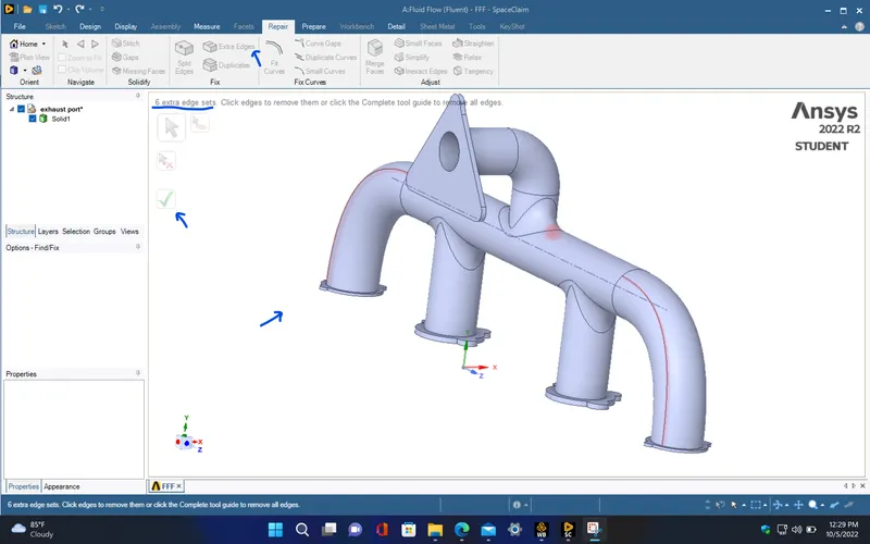
- Open spaceclaim from Ansys fluent flow and import the given exhaust port model into the spaceclaim. Then, to delete the extra edges that are present in the givel model, Use extra edges option under repair tab which automatically detects and removes the extra edges that are present.
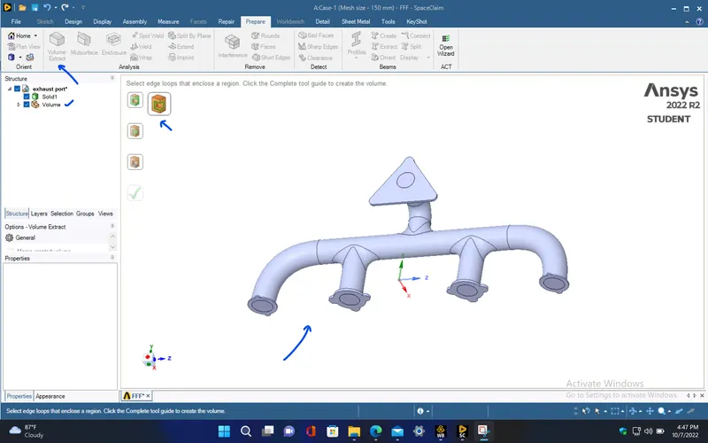
- Now, extract the fluid domain volume by selecting the necessary edges under volume extract option.
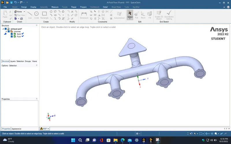
- Move the fluid and solid volume into a same single component in the structure tree and give a necessary name ot it.
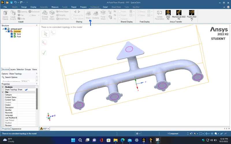
- Use the share topology option under workbench tab to share the common edges between the surfaces that are connected.
- Now, measure the required dimensions which can be used for calculating Y+ and heat transfer coefficient.
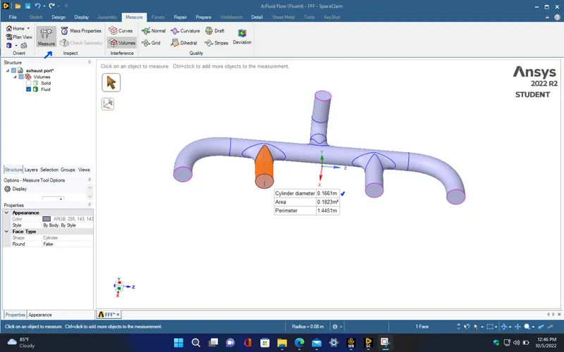
- Then, close the spaceclaim and open mesh window from the Ansys fluent flow. Give required names to the regions for which boundary conditions are to be given.
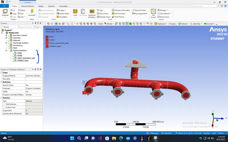
- To capture the geometry properly near to the surface where conjugate heat transfer occurs, create inflation layers with first layer thickness in that region. Therefore, to calculate the first layer thickness, Y+ value of 10 is used and since the fluid is air, the properties of air is given. Here, by giving those values, we get the first layer thickess of 0.6 mm.
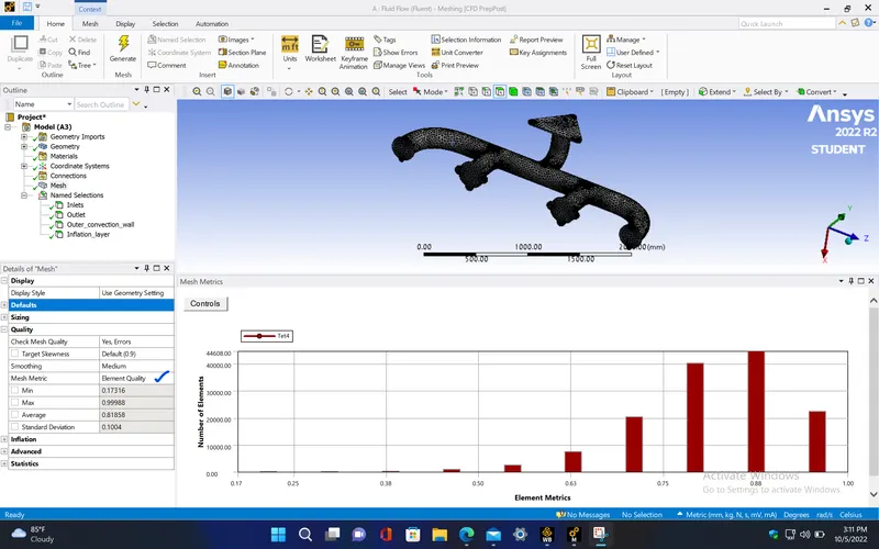
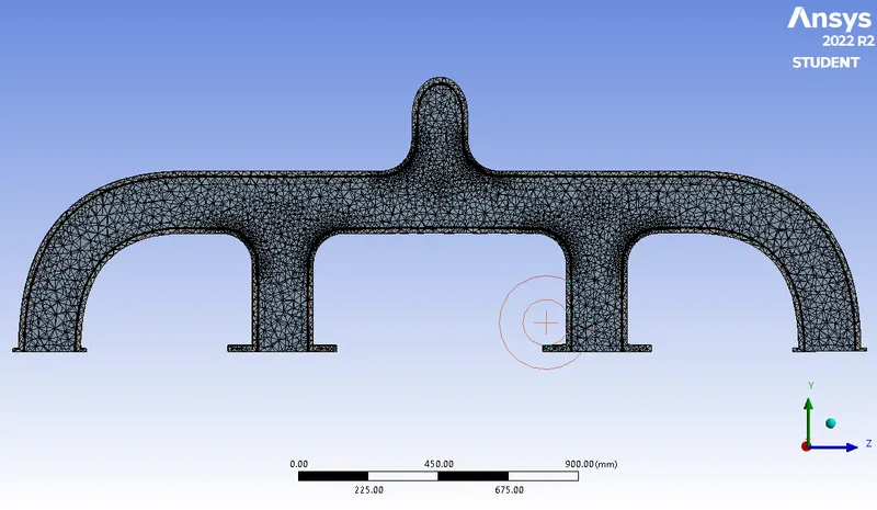
- Now, create the inflation layers with the first layer thickness of 0.6 mm and with maximum layers of 5 in the given named selection 'Inflation_layer'. Then, provide the mesh element size as 150 mm and generate mesh.
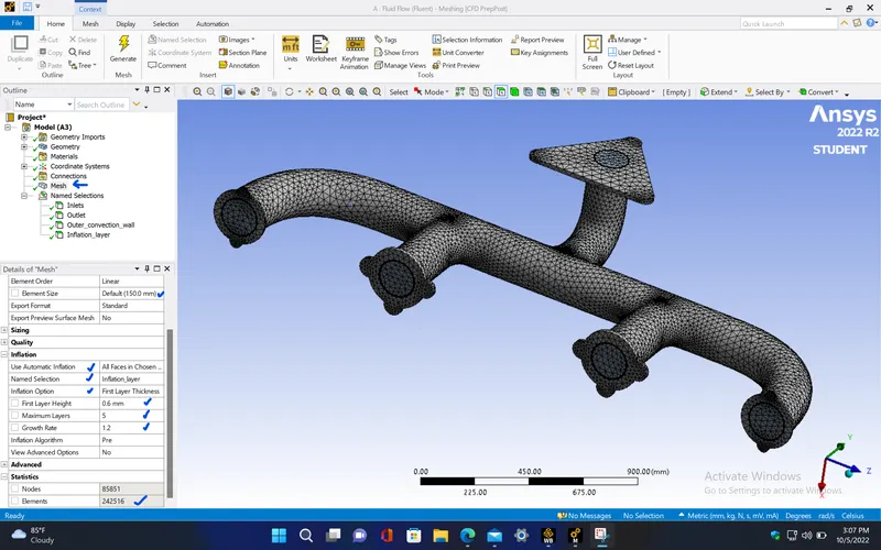
- Now, in order to check the mesh quality, under quality, choose mesh metric as element quality. Here, since most number of elements
|
Cells |
Faces |
Nodes |
|
242516 |
566614 |
92083 |
SETUP AND SOLVING :
- Setup the problem by selecting the required solver and boundary conditions for this simulation. The selected solver models and boundary conditions for running this simulation are as follows,
|
Model |
Settings |
|
Space |
3D |
|
Time |
Steady |
|
Viscous |
SST k-omega turbulence model |
|
Heat Transfer |
Enabled |
MATERIAL PROPERTIES :
|
Fluid |
air |
|
Density |
1.225 kg/m^3 |
|
Cp (Specific Heat) |
1006.43 J/(kg K) |
|
Thermal Conductivity |
0.0242 W/(m K) |
|
Viscosity |
1.7894e-05 kg/(m s) |
|
Molecular Weight |
28.966 kg/kmol |
|
Solid |
aluminum |
|
Density |
2719 kg/m^3 |
|
Cp (Specific Heat) |
871 J/(kg K) |
|
Thermal Conductivity |
202.4 W/(m K) |
BOUNDARY CONDITIONS :
|
inlets |
|
|
Velocity Specification Method |
Magnitude, Normal to Boundary |
|
Reference Frame |
Absolute |
|
Velocity Magnitude [m/s] |
5 |
|
Supersonic/Initial Gauge Pressure [Pa] |
0 |
|
Temperature [K] |
700 |
|
outlet |
|
|
Backflow Reference Frame |
Absolute |
|
Gauge Pressure [Pa] |
0 |
|
Backflow Total Temperature [K] |
300 |
|
Backflow Direction Specification Method |
Normal to Boundary |
|
Wall |
|
|
wall-volumes-solid |
|
|
Heat Generation Rate [W/m^3] |
0 |
|
Material Name |
aluminum |
|
Thermal BC Type |
Heat Flux |
|
Heat Flux [W/m^2] |
0 |
|
inflation_layer |
|
|
Heat Generation Rate [W/m^3] |
0 |
|
Material Name |
aluminum |
|
Thermal BC Type |
Coupled |
|
outer_convection_wall |
|
|
Heat Generation Rate [W/m^3] |
0 |
|
Material Name |
aluminum |
|
Thermal BC Type |
Convection |
|
Convective Heat Transfer Coefficient [W/(m^2 K)] |
20 |
|
Free Stream Temperature [K] |
300 |
|
inflation_layer-shadow |
|
|
Heat Generation Rate [W/m^3] |
0 |
|
Material Name |
aluminum |
|
Thermal BC Type |
Coupled |
|
Wall Motion |
Stationary Wall |
|
Shear Boundary Condition |
No Slip |
SOLVER :
|
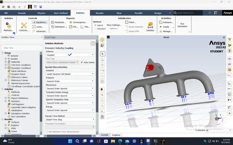
Pressure-Velocity Coupling |
Coupled |
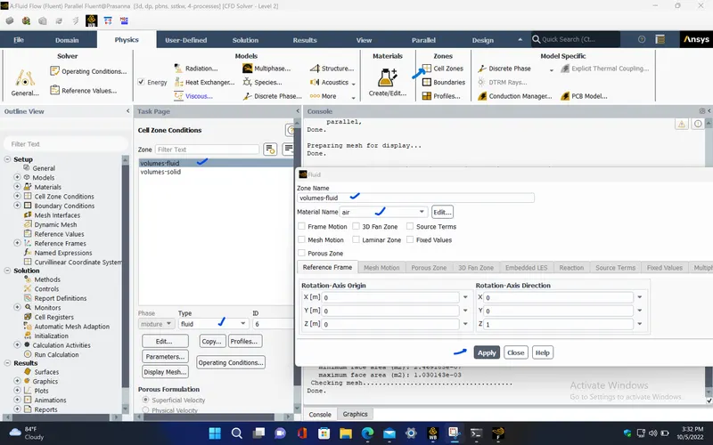
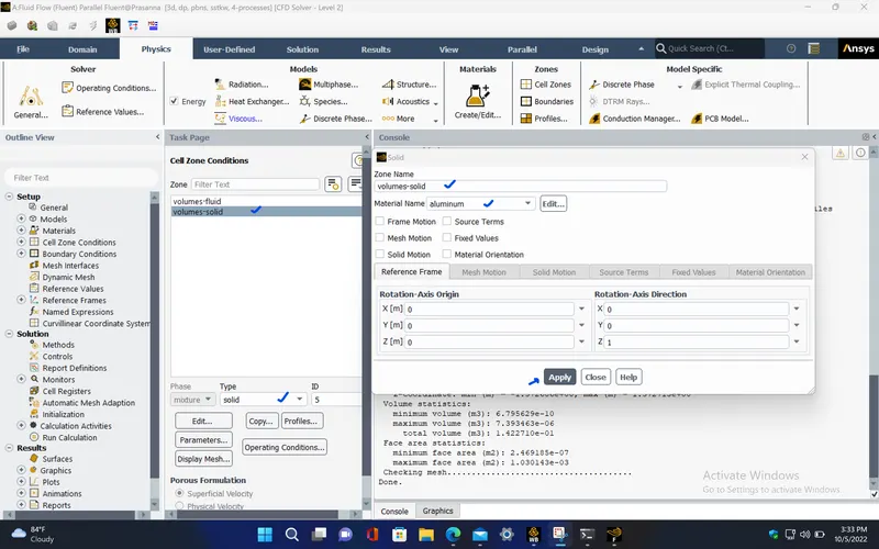
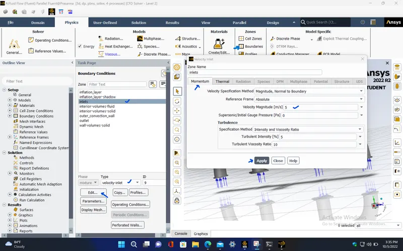
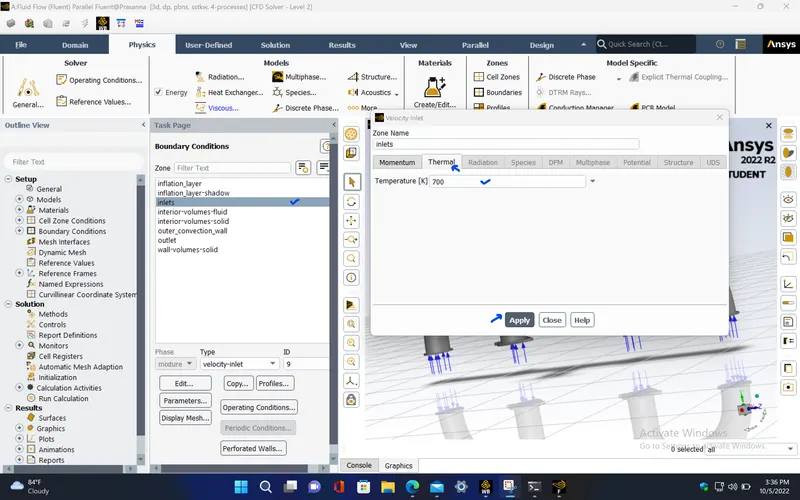
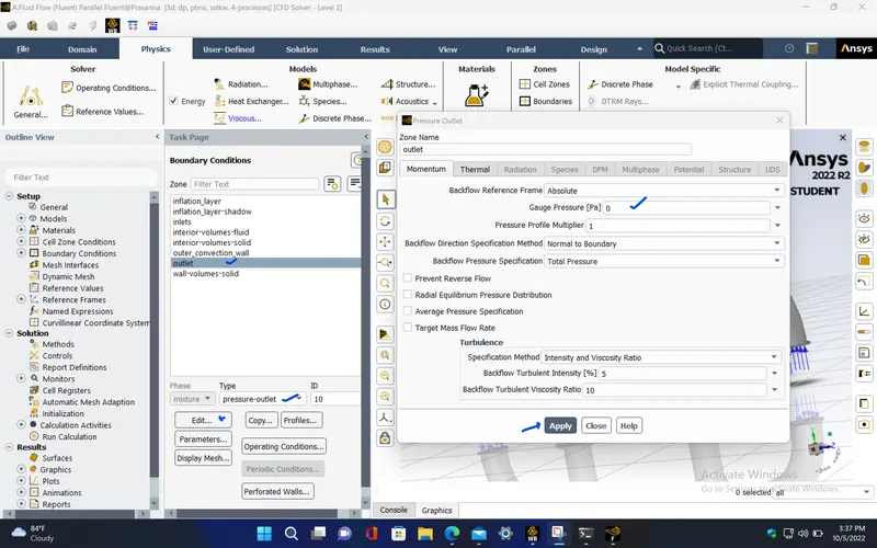
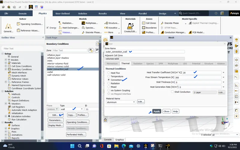
- Here, the outer wall is assumed to have a convective heat transfer of 20 W/m^2-K with the surrounding atmospheric air. Hence, the boundary condition for the outer convection wall is provided with the required thermal condition.
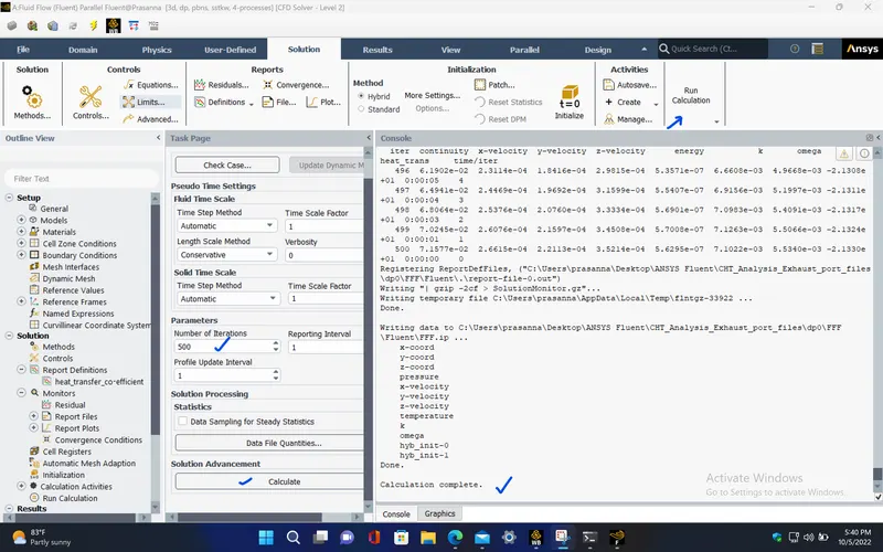
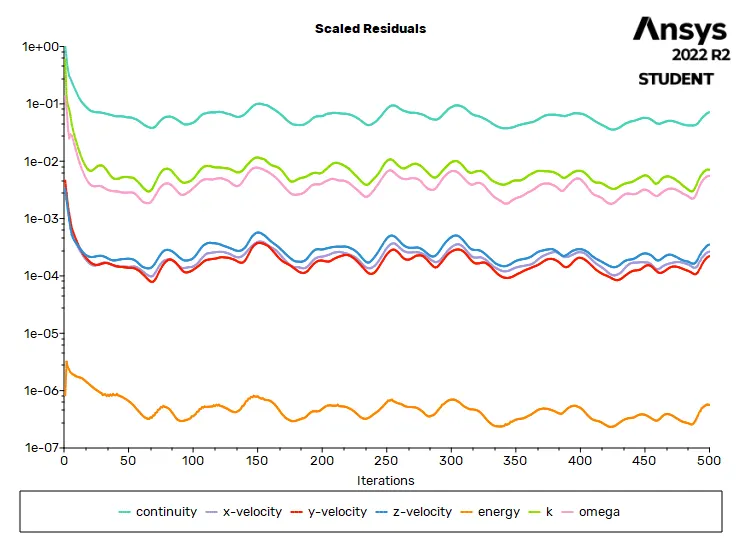
RESIDUALS PLOT :
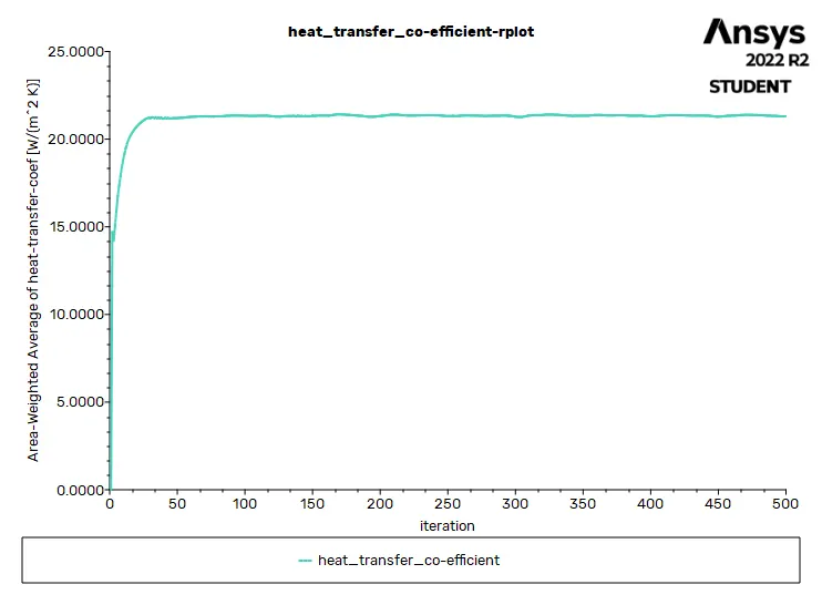
CONVECTIVE HEAT TRANSFER COEFFICIENT PLOT :
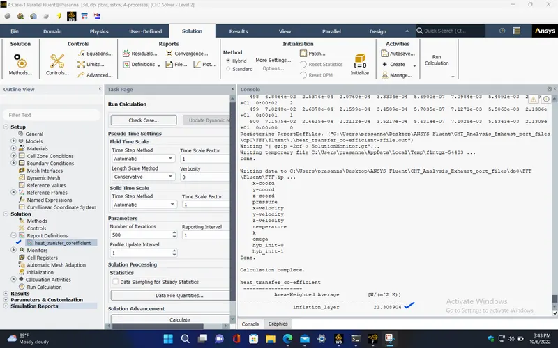
SOLUTION STATUS :
- From the above plots, we see that the solution got converged at 300th iteration since the rate at which residuals, velocity, drag co-efficient and lift co-efficient changes becomes constant over iteration.
Number of iteration - 500
|
Value |
Absolute Criteria |
Convergence Status |
|
|
continuity |
0.07157456 |
0.001 |
Not Converged |
|
x-velocity |
0.0002661468 |
0.001 |
Converged |
|
y-velocity |
0.0002211233 |
0.001 |
Converged |
|
z-velocity |
0.0003521743 |
0.001 |
Converged |
|
energy |
5.631447e-07 |
1e-06 |
Converged |
|
k |
0.007102782 |
0.001 |
Not Converged |
|
omega |
0.005534338 |
0.001 |
Not Converged |
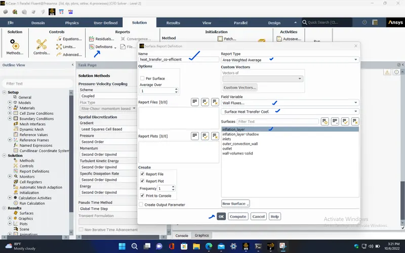
REPORT DEFINITIONS :
|
heat_transfer_co-efficient |
21.3089 |
W/(m^2 K) |
POST PROCESSING :
TEMPERATURE CONTOUR AT OUTER WALL :
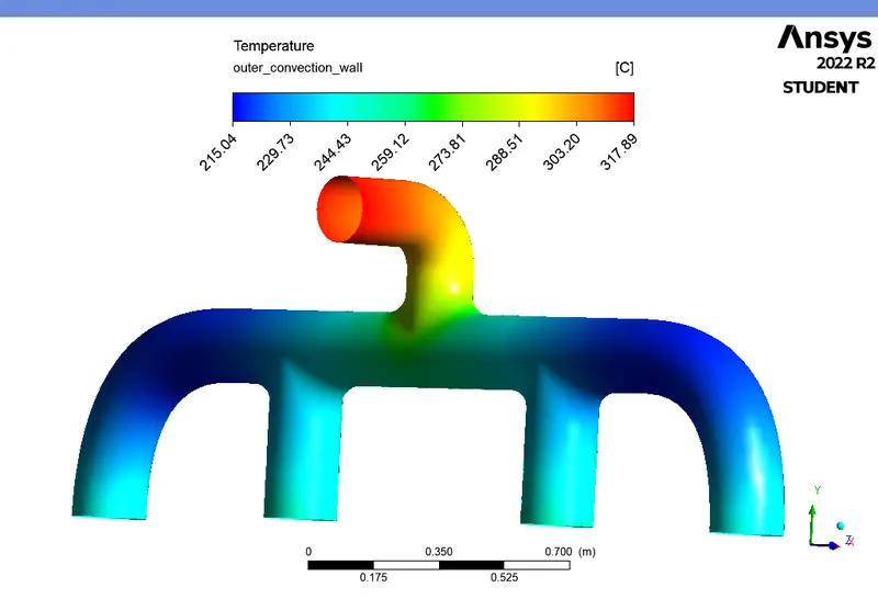
VELOCITY STREAMLINES :
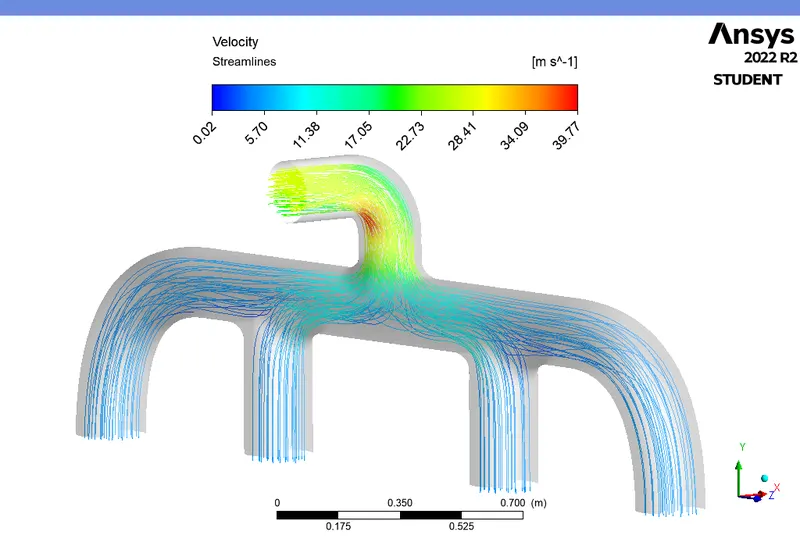
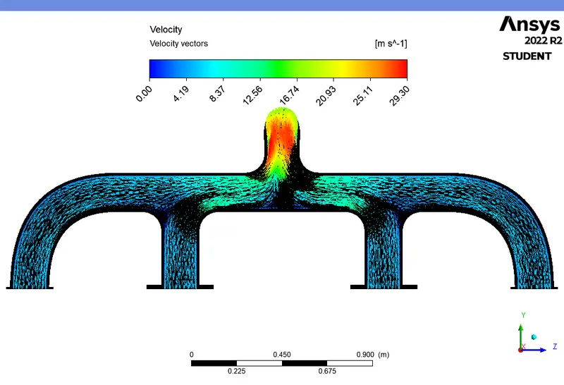
VELOCITY VECTORS AT YZ PLANE :
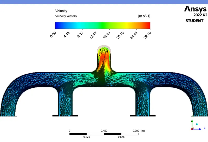
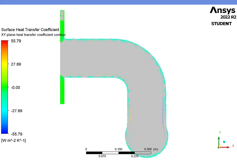
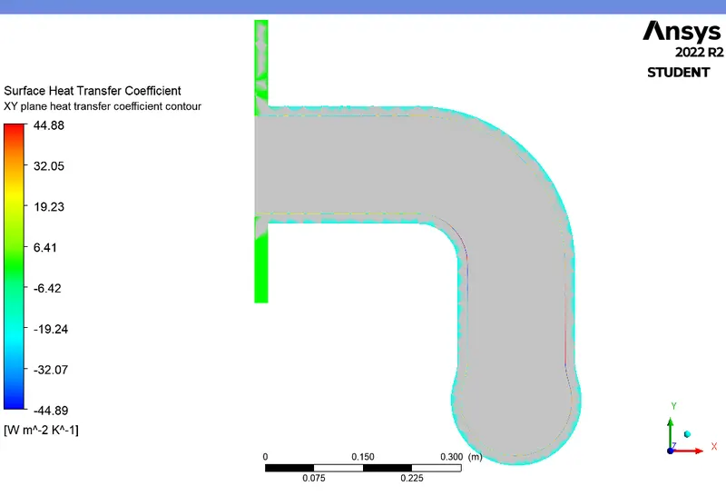
HEAT TRANSFER COEFFICIENT CONTOUR NEAR OUTLET :
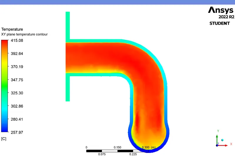
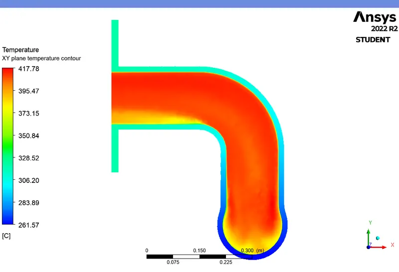
TEMPERATURE CONTOUR NEAR OUTLET :
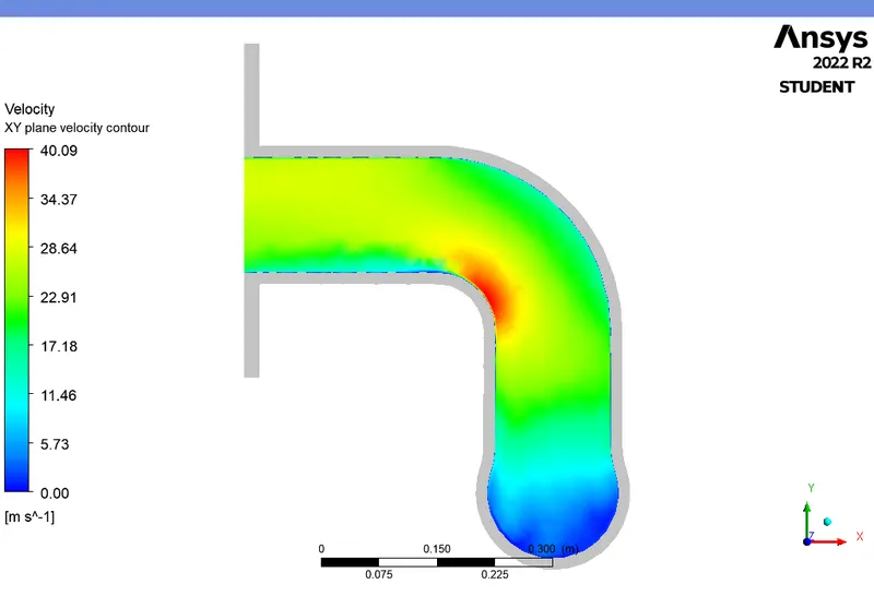
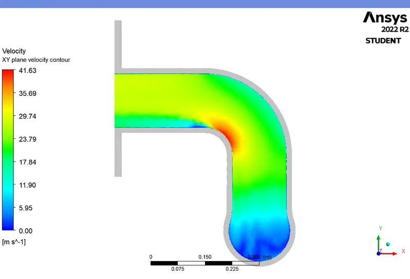
VELOCITY CONTOUR NEAR OUTLET :
CASE - 2 (Mesh element size - 50 mm, 20mm) :
PRE-PROCESSING :
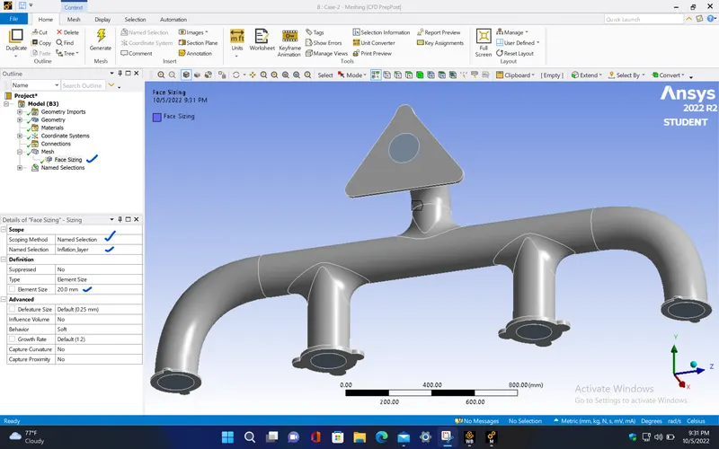
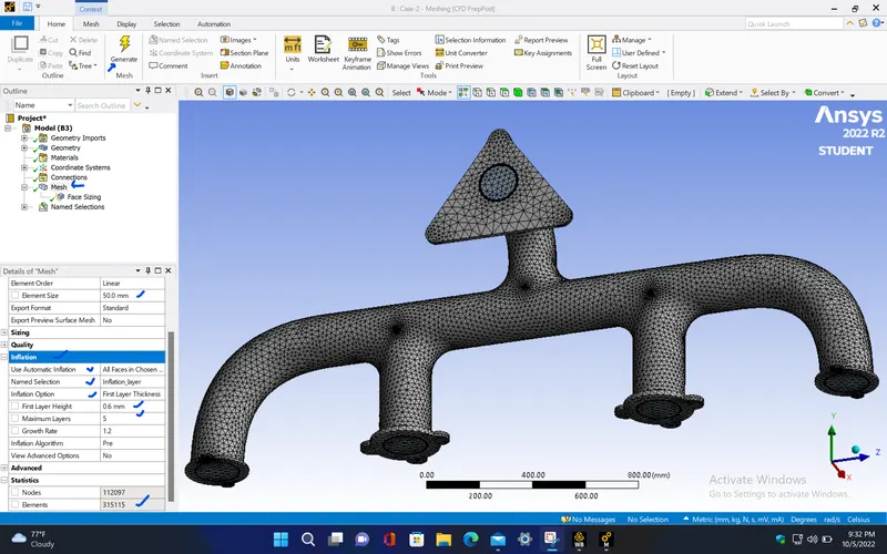
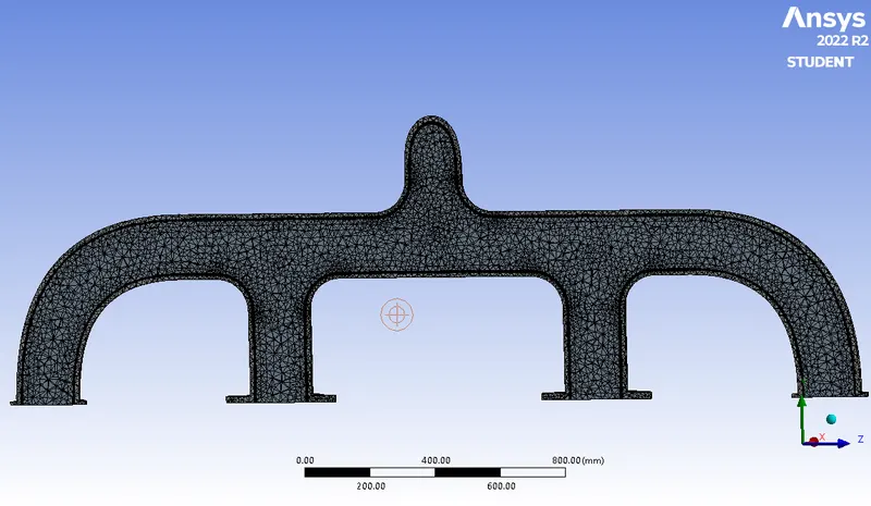
- Now change the mesh element size and also provide sizing for this case. Then, repeat the same procedure as done before.
|
Cells |
Faces |
Nodes |
|
315115 |
737359 |
120292 |
SETUP AND SOLVING :
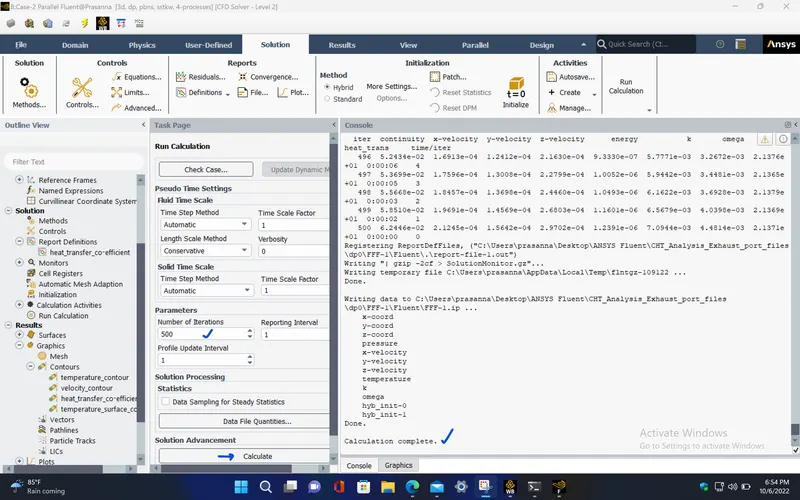
- Setup the problem by selecting the required solver and boundary conditions for this simulation. The selected solver models and boundary conditions for running this simulation are as follows,
|
Model |
Settings |
|
Space |
3D |
|
Time |
Steady |
|
Viscous |
SST k-omega turbulence model |
|
Heat Transfer |
Enabled |
MATERIAL PROPERTIES :
|
Fluid |
air |
|
Density |
1.225 kg/m^3 |
|
Cp (Specific Heat) |
1006.43 J/(kg K) |
|
Thermal Conductivity |
0.0242 W/(m K) |
|
Viscosity |
1.7894e-05 kg/(m s) |
|
Molecular Weight |
28.966 kg/kmol |
|
Solid |
aluminum |
|
Density |
2719 kg/m^3 |
|
Cp (Specific Heat) |
871 J/(kg K) |
|
Thermal Conductivity |
202.4 W/(m K) |
BOUNDARY CONDITIONS :
|
inlets |
|
|
Velocity Specification Method |
Magnitude, Normal to Boundary |
|
Reference Frame |
Absolute |
|
Velocity Magnitude [m/s] |
5 |
|
Supersonic/Initial Gauge Pressure [Pa] |
0 |
|
Temperature [K] |
700 |
|
outlet |
|
|
Backflow Reference Frame |
Absolute |
|
Gauge Pressure [Pa] |
0 |
|
Backflow Total Temperature [K] |
300 |
|
Backflow Direction Specification Method |
Normal to Boundary |
|
Wall |
|
|
wall-volumes-solid |
|
|
Heat Generation Rate [W/m^3] |
0 |
|
Material Name |
aluminum |
|
Thermal BC Type |
Heat Flux |
|
Heat Flux [W/m^2] |
0 |
|
inflation_layer |
|
|
Heat Generation Rate [W/m^3] |
0 |
|
Material Name |
aluminum |
|
Thermal BC Type |
Coupled |
|
outer_convection_wall |
|
|
Heat Generation Rate [W/m^3] |
0 |
|
Material Name |
aluminum |
|
Thermal BC Type |
Convection |
|
Convective Heat Transfer Coefficient [W/(m^2 K)] |
20 |
|
Free Stream Temperature [K] |
300 |
|
inflation_layer-shadow |
|
|
Heat Generation Rate [W/m^3] |
0 |
|
Material Name |
aluminum |
|
Thermal BC Type |
Coupled |
|
Wall Motion |
Stationary Wall |
|
Shear Boundary Condition |
No Slip |
SOLVER :
|
Pressure-Velocity Coupling |
Coupled |
RESIDUALS PLOT :
CONVECTIVE HEAT TRANSFER COEFFICIENT PLOT :
SOLUTION STATUS :
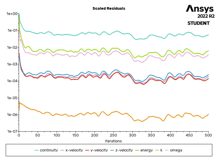
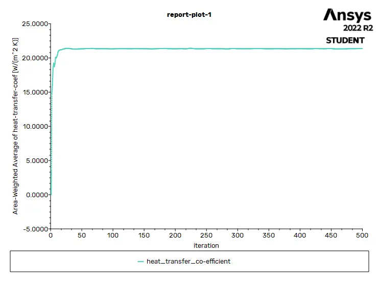
- From the above plots, we see that the solution got converged at 400th iteration since the rate at which residuals, velocity, drag co-efficient and lift co-efficient changes becomes constant over iteration.
Number of iteration - 500
|
Value |
Absolute Criteria |
Convergence Status |
|
|
continuity |
0.06244572 |
0.001 |
Not Converged |
|
x-velocity |
0.0002124512 |
0.001 |
Converged |
|
y-velocity |
0.0001564158 |
0.001 |
Converged |
|
z-velocity |
0.0002970169 |
0.001 |
Converged |
|
energy |
1.239138e-06 |
1e-06 |
Not Converged |
|
k |
0.007094388 |
0.001 |
Not Converged |
|
omega |
0.004481377 |
0.001 |
Not Converged |
REPORT DEFINITIONS :
|
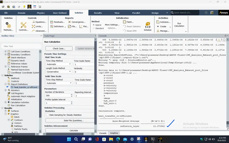
heat_transfer_co-efficient |
21.37096 |
W/(m^2 K) |
POST PROCESSING :
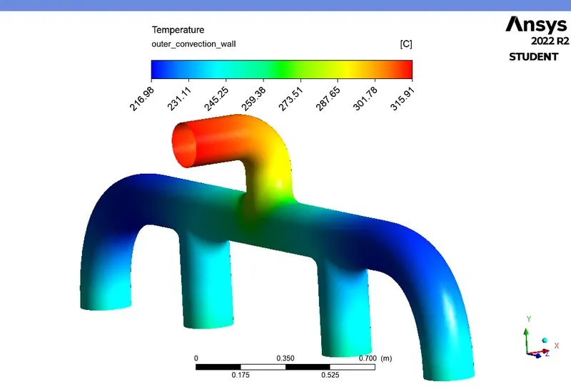
TEMPERATURE CONTOUR AT OUTER WALL :
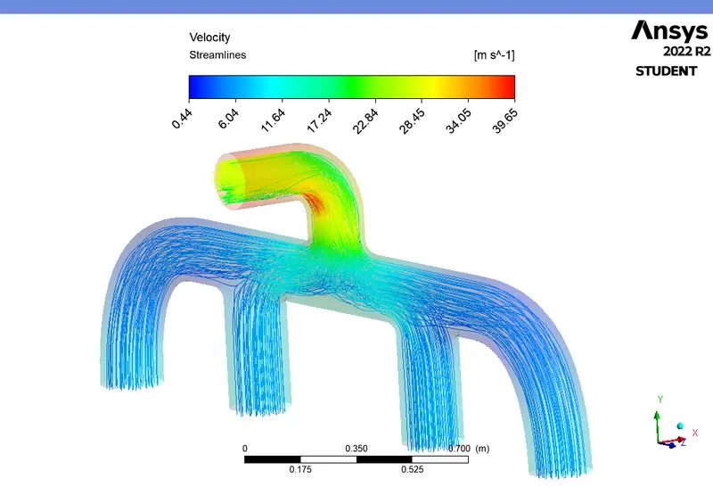
VELOCITY STREAMLINES :
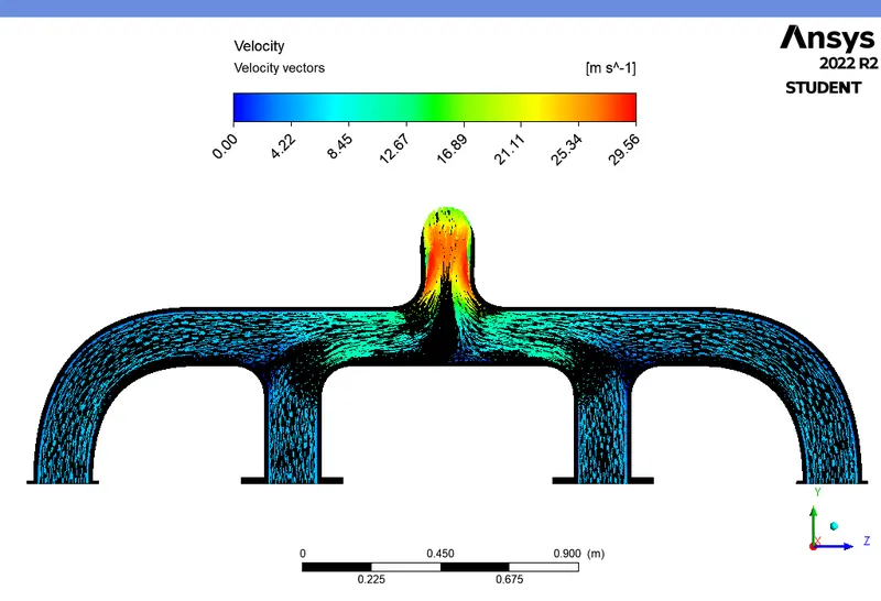
VELOCITY VECTORS AT YZ PLANE :
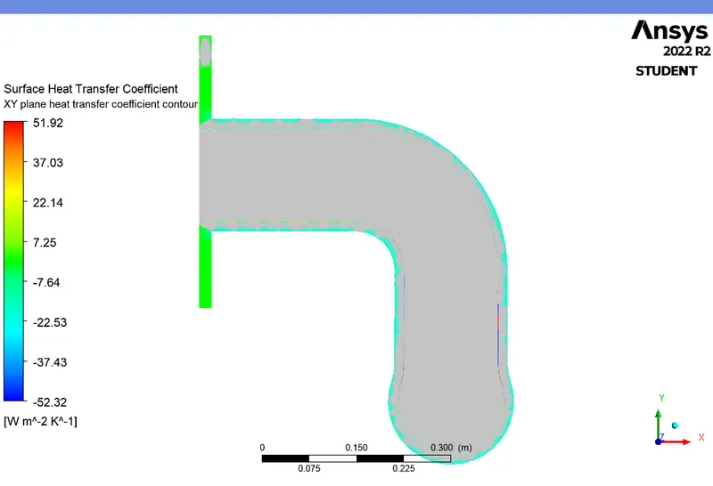
HEAT TRANSFER COEFFICIENT CONTOUR NEAR OUTLET :
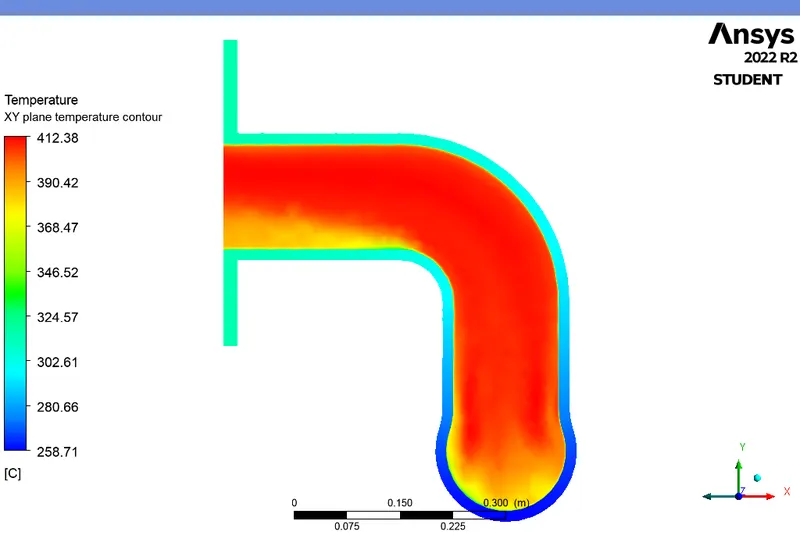
TEMPERATURE CONTOUR NEAR OUTLET :
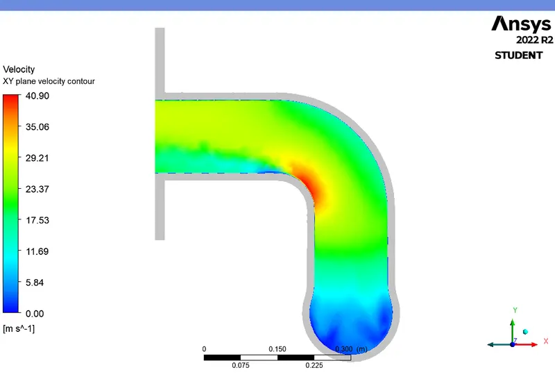
VELOCITY CONTOUR NEAR OUTLET :
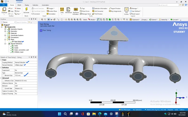
CASE - 3 (Mesh element size - 25 mm, 15mm) :
PRE-PROCESSING :
- Now change the mesh element size and also provide sizing for this case. Then, repeat the same procedure as done before.
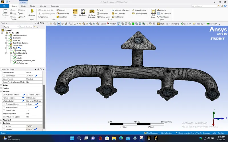
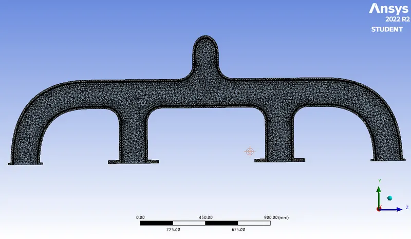
|
Cells |
Faces |
Nodes |
|
499010 |
1162923 |
187358 |
SETUP AND SOLVING :
- Setup the problem by selecting the required solver and boundary conditions for this simulation. The selected solver models and boundary conditions for running this simulation are as follows,
|
Model |
Settings |
|
Space |
3D |
|
Time |
Steady |
|
Viscous |
SST k-omega turbulence model |
|
Heat Transfer |
Enabled |
MATERIAL PROPERTIES :
|
Fluid |
air |
|
Density |
1.225 kg/m^3 |
|
Cp (Specific Heat) |
1006.43 J/(kg K) |
|
Thermal Conductivity |
0.0242 W/(m K) |
|
Viscosity |
1.7894e-05 kg/(m s) |
|
Molecular Weight |
28.966 kg/kmol |
|
Solid |
aluminum |
|
Density |
2719 kg/m^3 |
|
Cp (Specific Heat) |
871 J/(kg K) |
|
Thermal Conductivity |
202.4 W/(m K) |
BOUNDARY CONDITIONS :
|
inlets |
|
|
Velocity Specification Method |
Magnitude, Normal to Boundary |
|
Reference Frame |
Absolute |
|
Velocity Magnitude [m/s] |
5 |
|
Supersonic/Initial Gauge Pressure [Pa] |
0 |
|
Temperature [K] |
700 |
|
Turbulent Specification Method |
Intensity and Viscosity Ratio |
|
outlet |
|
|
Backflow Reference Frame |
Absolute |
|
Gauge Pressure [Pa] |
0 |
|
Backflow Total Temperature [K] |
300 |
|
Backflow Direction Specification Method |
Normal to Boundary |
|
Wall |
|
|
wall-volumes-solid |
|
|
Heat Generation Rate [W/m^3] |
0 |
|
Material Name |
aluminum |
|
Thermal BC Type |
Heat Flux |
|
Heat Flux [W/m^2] |
0 |
|
inflation_layer |
|
|
Heat Generation Rate [W/m^3] |
0 |
|
Material Name |
aluminum |
|
Thermal BC Type |
Coupled |
|
outer_convection_wall |
|
|
Heat Generation Rate [W/m^3] |
0 |
|
Material Name |
aluminum |
|
Thermal BC Type |
Convection |
|
Convective Heat Transfer Coefficient [W/(m^2 K)] |
20 |
|
Free Stream Temperature [K] |
300 |
|
inflation_layer-shadow |
|
|
Heat Generation Rate [W/m^3] |
0 |
|
Material Name |
aluminum |
|
Thermal BC Type |
Coupled |
|
Wall Motion |
Stationary Wall |
|
Shear Boundary Condition |
No Slip |
SOLVER :
|
Pressure-Velocity Coupling |
Coupled |
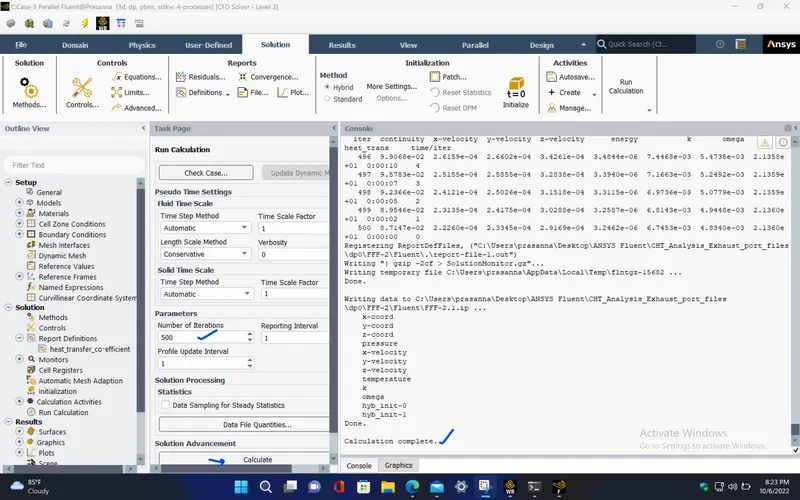
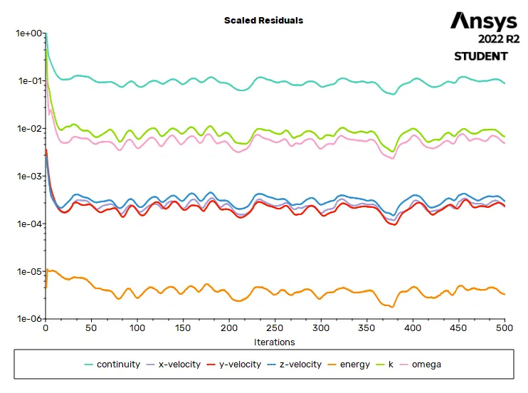
RESIDUALS PLOT :
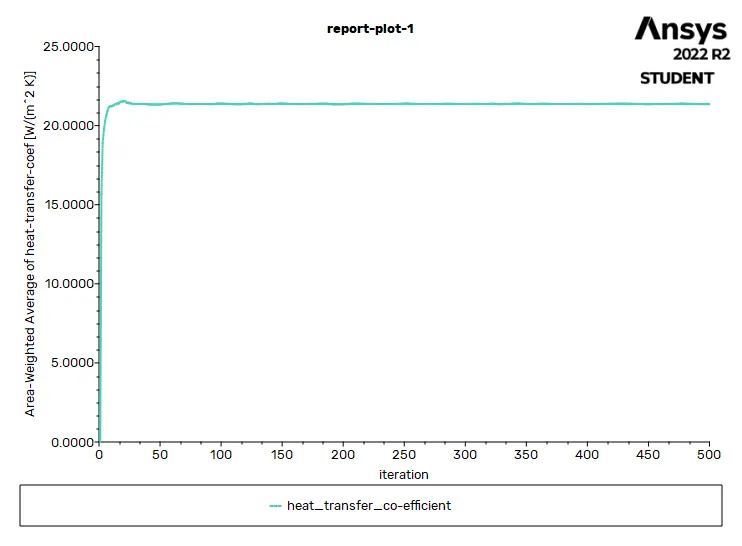
CONVECTIVE HEAT TRANSFER COEFFICIENT PLOT :
SOLUTION STATUS :
- From the above plots, we see that the solution got converged at 450th iteration since the rate at which residuals, velocity, drag co-efficient and lift co-efficient changes becomes constant over iteration.
Number of iteration - 500
|
Value |
Absolute Criteria |
Convergence Status |
|
|
continuity |
0.08714656 |
0.001 |
Not Converged |
|
x-velocity |
0.0002226036 |
0.001 |
Converged |
|
y-velocity |
0.0002334471 |
0.001 |
Converged |
|
z-velocity |
0.0002916927 |
0.001 |
Converged |
|
energy |
3.246155e-06 |
1e-06 |
Not Converged |
|
k |
0.006745344 |
0.001 |
Not Converged |
|
omega |
0.004833961 |
0.001 |
Not Converged |
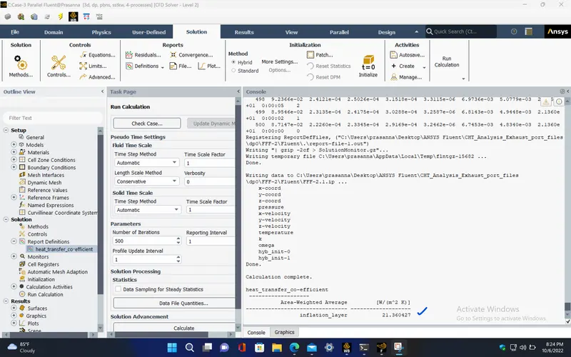
REPORT DEFINITIONS :
|
heat_transfer_co-efficient |
21.36043 |
W/(m^2 K) |
POST PROCESSING :
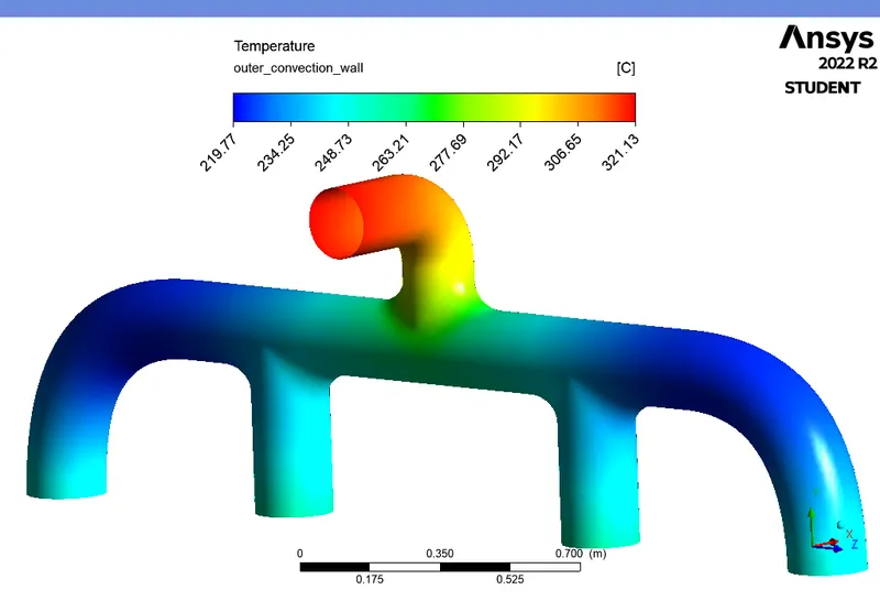
TEMPERATURE CONTOUR AT OUTER WALL :
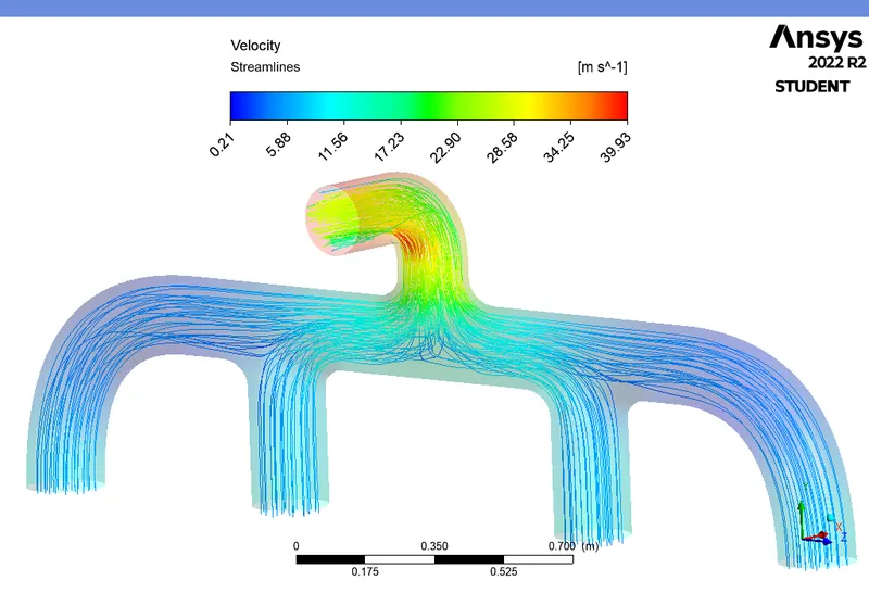
VELOCITY STREAMLINES :
VELOCITY VECTORS AT YZ PLANE :
HEAT TRANSFER COEFFICIENT CONTOUR NEAR OUTLET :
TEMPERATURE CONTOUR NEAR OUTLET :
VELOCITY CONTOUR NEAR OUTLET :
RESULTS :
Google drive link for the file :
https://drive.google.com/file/d/1coTYjmLsJrDsDQh58iM-REOFM2_-mXy4/view?usp=sharing
Mesh independency study :
|
|
MESH ELEMENT SIZE (in ‘mm’) |
Total Number of Mesh elements |
CONVECTIVE HEAT TRANSFER COEFFICIENT ( 'h' in ‘W/m^2 - K’) |
ERROR (%) |
||
|
Base mesh length |
Sizing |
SIMULATION RESULTS |
ANALYTICAL RESULTS |
|||
|
CASE - 1 |
150 |
- |
242516 |
21.3089 |
19.52 |
9.16 |
|
CASE - 2 |
50 |
20 |
315115 |
21.37096 |
19.52 |
9.48 |
|
CASE - 3 |
25 |
15 |
499010 |
21.36043 |
19.52 |
9.43 |
CONCLUSION :
From the above table, we can observe that the difference between the simulation results for different cases doesn't vary much. Hence, the Case - 1 which has less number of mesh elements gives the simulation result in less computatational time than other cases, so it can be taken as a refined mesh length for this simulation.
Accuracy of HTC prediction :
Accuracy of the predictions depends mainly upon,
- Accurate geometry of the model.
- Choosing a proper mesh size and improving the mesh quality.
- Creating the inflation layers near to the boundary region where the heat transfer occurs.
- Choosing the correct turbulence models.
- Providing the correct values for the material's properties.
VELOCITY CONTOUR NEAR OUTLET :
HEAT TRANSFER COEFFICIENT CONTOUR NEAR OUTLET :
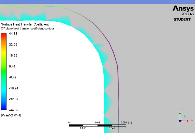
- From the above contour plots, we can conclude that the heat transfer co-efficeint is higher in the region where the velocity is high. Since according to the mass conservation, we know that the total mass entering must be equal to total mass leaving at outlet of the exhaust port, the amount of air flowing through all the inlet pipes are combined into a single pipe, where the mass flow rate is higher and so the velocity. This increase in velocity of air increases the heat transfer rate at that region and hence the convective heat transfer coefficient is high in that region.