Project 2 - Rankine cycle Simulator

AIM:- Rankine Cycle Simulator

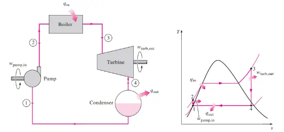
Introduction:- A Rankine cycle is an idealized Thermodynamic cycle that governs the working of a Heat Engine. In the Rankine cycle, the friction losses of a heat engine are neglected. It is a cycle that converts heat into mechanical energy which usually is converted into electrical energy. There are four components in this cycle that work on four different processes. The four components are the turbine, Condensor, Pump, and Boiler. The Rankine cycle is nothing but a modification of the Carnot cycle. The ideal Rankine cycle is very useful in steam power plants and gas power plants. To improve the efficiency of the Rankine cycle in the steam power plant, there are some changes in the Rankine cycle that differs from the Carnot cycle. Firstly, a pump is used in place of a condenser to handle only liquid, not a mixture of liquid and vapor. Secondly, exhaust steam from the turbine is completely condensed in the condenser.

The process in the Rankine cycle is given as:

1. Isentropic Compression in Pump.
2. Constant pressure heat addition in the boiler.
3. Isentropic expansion in a turbine.
4. Constant pressure heat rejection in the condenser.

Rankine cycle efficiency ηR is -

Back Work Ratio:

The fraction of the work produced by the turbine that is consumed by the compressor.

BW ratio=Wp/Wt

Explanation:

1. The creation of the Rankine cycle simulator starts with some input values which is required to calculate the other state point in the cycle eventually.
2. The Rankine cycle process is displayed in the command window and then inputs are entered which are inlet pressure for the turbine, temperature at the turbine inlet, and pressure at the condenser.
3. Then we are using the XStream function file for reading the state point. First, we get the value of enthalpy and entropy at state point 1 from the XStream function file.
4. As process from 1-2 is isentropic compression the entropy at point 1 is equal to point 2. The term ‘(s_pT, p1, T1)’ refers to entropy at pressure and temperature point 1.
5. The term ‘sg’ and ‘sf’ are referred to saturated liquid and saturated vapor entropy respectively. This value is used to calculate other functions according to mathematical relations.
6. Similarly, other points are taken from the XStream function file which is necessary to calculate other parameters. After that work done in the turbine and pump is calculated for further getting the net work done Rankine cycle.
7. After calculating the net work done the efficiency of the Rankine cycle is calculated along with specific steam consumption which is steam consumed by a locomotive cylinder per unit of output of work done.
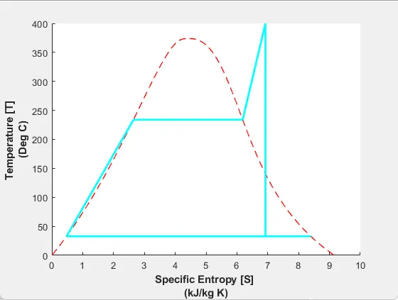
8. The temperature at each point of the cycle is calculated using input taken from the start of the program and data taken from the XStream file. For a given temperature range from lower to higher entropy points are calculated to create the T-S plot. Similarly, another for loop is used to create the saturation curve in each plot.
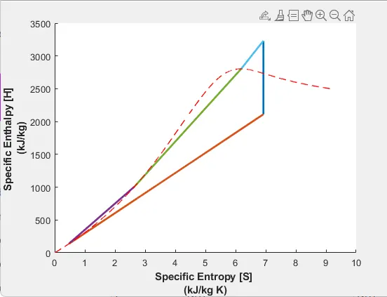
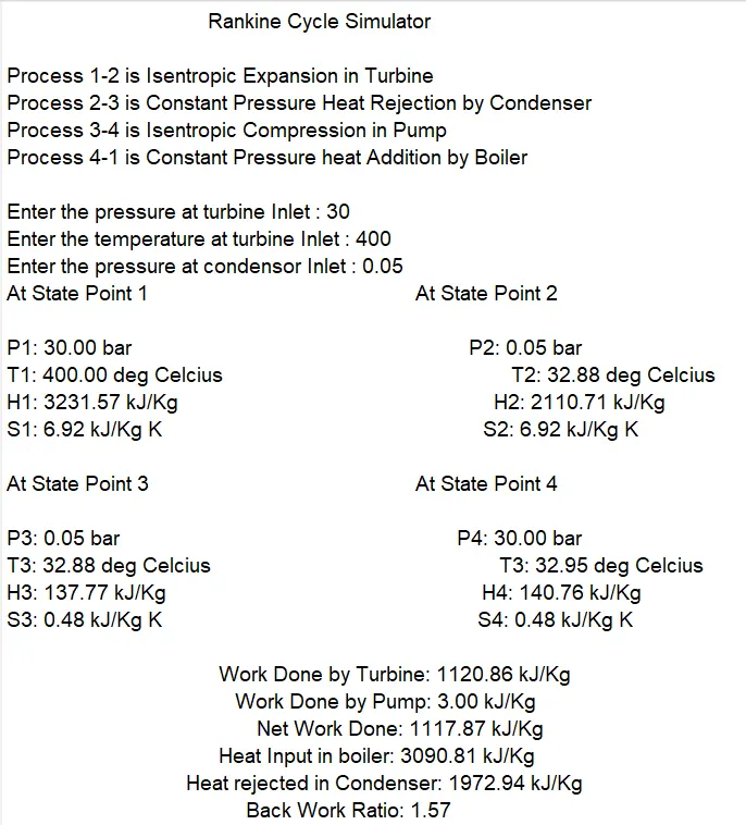
9. Then plotting is done respectively for T-s and H-s graphs in the Rankine cycle and each state point value has been put in the command window.

The code for Rankine Cycle Simulator is given as:

MATLAB Code:-

clear all % Clears command history

close all % Closes all windows

clc % Clears command window

% Basic Info

fprintf('%60s \r\n', 'Rankine Cycle Simulator')

fprintf('%s \n','Process 1-2 is Isentropic Expansion in Turbine')

fprintf('%s \n','Process 2-3 is Constant Pressure Heat Rejection by Condenser')

fprintf('%s \n','Process 3-4 is Isentropic Compression in Pump')

fprintf('%s \r\n','Process 4-1 is Constant Pressure heat Addition by Boiler')

%% INPUTS

p1=input('Enter the pressure at turbine Inlet : ');

t1=input('Enter the temperature at turbine Inlet : ');

p2=input('Enter the pressure at Condensor Inlet : ');

%% 1-2 Isentropic Turbine Expansion

h1=XSteam('h_pT',p1,t1);

s1=XSteam('s_pT',p1,t1);

tsat1=XSteam('Tsat_p',p1); %Saturation Temp.at p1

hg1=XSteam('hV_p',p1);

hf1=XSteam('hL_p',p1);

sg1=XSteam('sV_p',p1);

sf1=XSteam('sL_p',p1);

s2=s1;

hf2=XSteam('hL_p',p2);

sf3=XSteam('sL_p',p2);

hg2=XSteam('hV_p',p2);

sg2=XSteam('sV_p',p2);

sfg=sg2-sf3; %entropy of wet region

hfg= hg2-hf2;

if s2 < sg2 % Checks to see if Point 2 is within the vapor dome

x2=(s2-sf3)/sfg; % calculates the new quality at this point

h2=hf2+x2*hfg; % calculates the new enthalpy

else

x2 = 1; % Quality is max 1

h2 = x2*hg2; % calculates the new enthalpy

end

t2=XSteam('T_ps',p2,s2);

tsat2=XSteam('Tsat_p',p2); %Saturation Temp.at p2

%% 2-3 Isobaric Condenser

p3=p2;

s3=sf3;

h3=hf2;

%% 3-4 Isentropic Pump

s4=s3;

t3=tsat2;

%% 4-1 Isobaric Boiler

p4=p1;

h4=XSteam('h_ps',p4,s4);

t4=XSteam('T_ps',p4,s4);

%% T-S & H-S Diagrams

t= linspace(1,t1,5000);

figure(1)

%axis([1.91984 1.92 157.4 158.3]);

hold on

sl=zeros;

sv=zeros;

hl=zeros;

hv=zeros;

for i=1:length(t)

sl(i)=XSteam('sL_T',t(i));

sv(i)=XSteam('sV_T',t(i));

hl(i)=XSteam('hL_T',t(i));

hv(i)=XSteam('hV_T',t(i));

end

plot(sl,t,'--r','linewidth',1)

plot(sv,t,'--r','linewidth',1)

%% T-S Diagram Animation

for i=s1:s2

a=linspace(s1,s2,100);

b=linspace(t1,t2,100);

curve=animatedline('color','c','linewidth',2);

for j=1:100

x=a(j);

y=b(j);

addpoints(curve,x,y);

pause(0.01) ;

end

end

for i=sg2:s2

a=linspace(s2,sg2,100);

b=linspace(t2,tsat2,100);

curve=animatedline('color','c','linewidth',2);

for j=1:100

x=a(j);

y=b(j);

addpoints(curve,x,y);

pause(0.01) ;

end

end

for i=s3:sg2

a=linspace(sg2,s3,100);

b=linspace(tsat2,t3,100);

curve=animatedline('color','c','linewidth',2);

for j=1:100

x=a(j);

y=b(j);

addpoints(curve,x,y);

pause(0.01) ;

end

end

for i=s3:s4

a=linspace(s3,s4,100);

b=linspace(t3,t4,100);

curve=animatedline('color','c','linewidth',2);

for j=1:100

x=a(j);

y=b(j);

addpoints(curve,x,y);

pause(0.01) ;

end

end

for i=s4:sf1

a=linspace(s4,sf1,100);

b=linspace(t4,tsat1,100);

curve=animatedline('color','c','linewidth',2);

for j=1:100

x=a(j);

y=b(j);

addpoints(curve,x,y);

pause(0.01) ;

end

end

for i=sf1:sg1

a=linspace(sf1,sg1,100);

b=linspace(tsat1,tsat1,100);

curve=animatedline('color','c','linewidth',2);

for j=1:100

x=a(j);

y=b(j);

addpoints(curve,x,y);

pause(0.01) ;

end

end

for i=sg1:s1

a=linspace(sg1,s1,100);

b=linspace(tsat1,t1,100);

curve=animatedline('color','c','linewidth',2);

for j=1:100

x=a(j);

y=b(j);

addpoints(curve,x,y);

pause(0.01) ;

end

end

%

%plot([s1 s2],[t1 t2],'linewidth',2)

%plot([s2 sg2],[t2 tsat2],'linewidth',2)

%plot([sg2 s3],[tsat2 t3],'linewidth',2)

%plot([s3 s4],[t3 t4],'linewidth',2)

%plot([s4 sf1],[t4 tsat1],'linewidth',2)

%plot([sf1 sg1],[tsat1 tsat1],'linewidth',2)

%plot([sg1 s1],[tsat1 t1],'linewidth',2)

xlabel({'Specific Entropy [S] ','(kJ/kg K)'},'FontWeight','bold')

ylabel({'Temperature [T] ','(Deg C)'},'FontWeight','bold')

%% H-S Diagram Animation

figure(2)

hold on

plot([s1 s2],[h1 h2],'linewidth',2)

plot([s2 s3],[h2 h3],'linewidth',2)

plot([s3 s4],[h3 h4],'linewidth',2)

plot([s4 sf1],[h4 hf1],'linewidth',2)

plot([sf1 sg1],[hf1 hg1],'linewidth',2)

plot([sg1 s1],[hg1 h1],'linewidth',2)

plot([sl sv],[hl hv],'--r','linewidth',1)

xlabel({'Specific Entropy [S] ','(kJ/kg K)'},'FontWeight','bold')

ylabel({'Specific Enthalpy [H] ' ,'(kJ/kg)'},'FontWeight','bold')

%% Efficiency and Work

Wt=h1-h2;

Wp=h4-h3;

W=Wt-Wp;

qin=h1-h4;

qout=h2-h3;

eff=W*100/qin;

bwr=qin/qout;

%% Display

fprintf('%-60s %20s \r\n', 'At State Point 1','At State Point 2' )

fprintf('%s %.2f %s %64s %.2f %s \n','P1:',p1,'bar','P2:',p2,'bar')

fprintf('%s %.2f %s %55s %.2f %s \n','T1:',t1,'deg Celcius','T2:',t2,'deg Celcius')

fprintf('%s %.2f %s %60s %.2f %s \n','H1:',h1,'kJ/Kg','H2:',h2,'kJ/Kg')

fprintf('%s %.2f %s %61s %.2f %s \r\n','S1:',s1,'kJ/Kg K','S2:',s2,'kJ/Kg K')

fprintf('%-60s %20s \r\n', 'At State Point 3','At State Point 4' )

fprintf('%s %.2f %s %64s %.2f %s \n','P3:',p3,'bar','P4:',p4,'bar')

fprintf('%s %.2f %s %55s %.2f %s \n','T3:',t3,'deg Celcius','T3:',t4,'deg Celcius')

fprintf('%s %.2f %s %60s %.2f %s \n','H3:',h3,'kJ/Kg','H4:',h4,'kJ/Kg')

fprintf('%s %.2f %s %60s %.2f %s \r\n','S3:',s3,'kJ/Kg K','S4:',s4,'kJ/Kg K')

fprintf('%60s %.2f %s \n','Work Done by Turbine:',Wt,'kJ/Kg')

fprintf('%60s %.2f %s \n','Work Done by Pump:',Wp,'kJ/Kg')

fprintf('%60s %.2f %s \n','Net Work Done:',W,'kJ/Kg')

fprintf('%60s %.2f %s \n','Heat Input in boiler:',qin,'kJ/Kg')

fprintf('%60s %.2f %s \n','Heat rejected in Condenser:',qout,'kJ/Kg')

fprintf('%60s %.2f \n','Back Work Ratio:',bwr)

Output:-