Plot otto cycle piston kinematics p-v diagram in matlab

• Aim : Plot otto cycle piston kinematics p-v diagram in matlab

• Objective: Write a program to solve piston kinematic equation How does volume and pressure change in combustion chamber
• Explanation:

First we take inputs variables like gamma, temperature, pressure and also engine geometric parameters like bore, stroke, connecting rod length , compression ratio .

Then we calculate swept and clearance volume using formulae

Swept volume=(π4)⋅bore2⋅stroke

Clearance volume = swept_v/(cr-1)

then we calculate volume (1) and volume (2) of cylinder using equations

then we calculate pressure at stage (2)

p2=p1*cr^gamma

then using above values we calculate temperature at stage 2

t2= p2*v2*t1/(p1*v1)

then we use function command engine kinematics and putting values in it then we get curve line at point one to two. The process involved at point one to two is isentropic compression.

constant_c = p1*v1^gamma

P_compression = constant_c./V_compression.^gamma

The process from point 2 to 3 is constant volume heat addition. In this process volume is same v2=v3 so we calculate p3 using obtain values

P3= p2*t3/t2

then we use function command engine kinematics and putting values in it then we get curve line at point one to two. The process involved at point one to two is isentropic expansion.

constant_c = p3*v3^gamma;

P_expansion = constant_c./V_expansion.^gamma;

The process from point 2 to 3 is constant volume heat rejection. In this process volume is same v4=v1 so we calculate p4 using obtain values .

Then lastly plot the figure using red colour and giving label volume and pressure

clear all
close all
clc
% input variables
gamma = 1.4
t3 = 2300

% state variables
p1 = 101325
t1 = 500


% Engine geometric parameters
bore = 0.1;
stroke = 0.1;
connecting_rod = 0.15;
cr = 12;

% calculating the swept volume and the clearance volume

swept_v = (pi/4)*bore^2*stroke;
clearance_v = swept_v/(cr-1);


v1 = swept_v + clearance_v
v2 = clearance_v

 % state variables at state point 2
 % p2v2^gamma = p1v1^gamma
 % p2 = p1*(v1/v2)^gamma = p1*cr^gamma

 p2 = p1*cr^gamma;

 % p1v1/t1 = p2v2/t2 | t2 = p2*v2*t1/(p1*v1)

 t2 = p2*v2*t1/(p1*v1);

 constant_c = p1*v1^gamma;
 V_compression = engine_kinematics(bore,stroke,connecting_rod,cr,180,0)

P_compression = constant_c./V_compression.^gamma 



 % state variables at state point 3
 v3 = v2




 % p3v3/t3 = p2v2/t2 |  p3 = p2*t3/t2

  p3 = p2*t3/t2

  constant_c = p3*v3^gamma;
 V_expansion = engine_kinematics(bore,stroke,connecting_rod,cr,0,180)

P_expansion = constant_c./V_expansion.^gamma;


% state variables at state point 4
v4 = v1

%p3v3^gamma = p4v4^gamma | p4 = p3(v3/v4)^gamma

p4 = p3*(v3/v4)^gamma





figure(1)
hold on
plot (v1,p1,'*','color','r')
plot(V_compression,P_compression)
plot (v2,p2,'*','color','r')
plot (v3,p3,'*','color','r')
plot(V_expansion,P_expansion)
plot (v4,p4,'*','color','r')
plot([v3 v2],[p3 p2])
plot([v4 v1],[p4 p1])
xlabel('Volume')
ylabel('Pressure')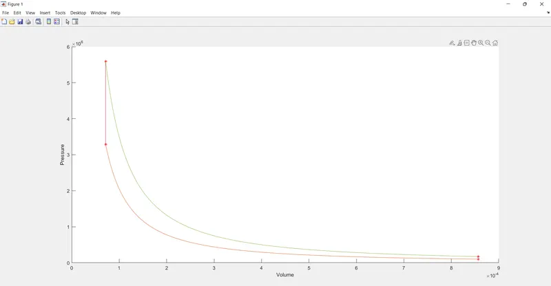

OUTPUT

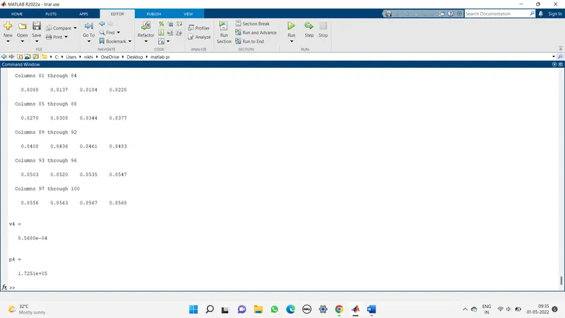
COMMAND WINDOW

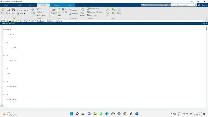
COMMAND WINDOW