Week 4.1 - Genetic Algorithm

• Aim : to find the global maxima for the stalagmite function using Ga in matlab.
• Explanation :
• GA (Genetic Algorithm) :

It is a numerical method in that this solves unconstrained optimization problem . It repeatedly modifies a population in individual solution. At each step Ga randomly select individual from the current population and uses them as parent to produced the children for the next generation

There are in GA 3 main types

1. Selection: rules select the individual called parents that contributes the population at the next generation.
2. Crossover: rules combine two parents to form children for next generation.
3. Mutation : rules apply random changes to individual parents to form children.

Process of natural selection

1.initial population: The process begins with a set of individuals which is called a Population. Each individual is a solution to the problem you want to solve. An individual is characterized by a set of parameters (variables) known as Genes. Genes are joined into a string to form a Chromosome (solution). In a genetic algorithm, the set of genes of an individual is represented using a string, in terms of an alphabet. Usually, binary values are used (string of ls and Os). We say that we encode the genes in a chromosome.

2.Fitness function:Fitness Function (also known as the Evaluation Function) evaluates how close a given solution is to the optimum solution of the desired problem. It determines how fit a solution is.

• why we use fitness functions: In genetic algorithms, each solution is generally represented as a string of binary numbers, known as a chromosome. We have to test these solutions and come up with the best set of solutions to solve a given problem. Each solution, therefore, needs to be awarded a fitness score, to indicate how close it came to meeting the overall specification of the desired solution. This score is generated by applying the fitness function to the test, or results obtained from the tested solution.

3.Selection: The selection is based on the fitness score. The idea of selection phase is to select the fittest individuals and let them pass their genes to the next generation. Two pairs of individuals (parents) are selected based on their fitness scores. Individuals with high fitness have more chance to be selected for reproduction

4.Crossover: Crossover is the most significant phase in a genetic algorithm. For each pair of parents to be mated, a crossover point is chosen at random from within the genes. Offspring are created by exchanging the genes of parents among themselves until the crossover point is reached.

5. Mutation: In certain new offspring formed, some of their genes can be subjected to a mutation with a low random probability. This implies that some of the bits in the bit string can be flipped. Mutation occurs to maintain diversity within the population and prevent premature convergence. termination The algorithm terminates if the population has converged (does not produce offspring which are significantly different from the previous generation).

Following statements to summerize how work Genetic Algorithm.

1. It starts with creating random initial population.
2. Then it creates a sequence of new populations. At each step , algorithm uses individuals of current generation
3. The algorithm stops when one of the stopping criteria is met

What is stalagmite ?

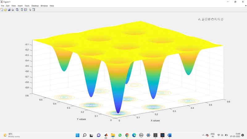
It is the mathematical model which helps to generate local minimum and maximas which is 3 dimensional.

Program Explanation :

clear all

close all

clc

% defining our search space

x = linspace(0,0.6,150);

y = linspace(0,0.6,150);

num_cases = 50;

first we takes values of x and y i.e. 150 and the values are in between 0 to 0.6 and also conder no. of iteration num_cases: 50

then we forming array i.e 2 dimensional using meshgrid and for loop

[xx yy] = meshgrid(x,y);

for i = 1:length(xx)

for j = 1:length(yy)

input_vector(1) = xx(i,j);

input_vector(2) = yy(i,j);

f(i,j) = stalagmite(input_vector);

end

end

Since we need to plot a 3D surface plot we take the 2d array of x and y using meshgrid command and store them in input_vector array so that it can be used as an argument to call the function

stalagmite

we create another function file for the stalagmite function. here we take the output as -f since Ga only minimises a given function. so if -f is considered it automatically gives us the maxima.

function f = stalagmite(input_vector)

x = input_vector(1);

y = input_vector(2);

f1 = (sin(5.1*pi*x+0.5))^6;

f2 = (sin(5.1*pi*y+0.5))^6;

f3 = exp((-4*log(2)*(x-0.0667)^2)/0.64);

f4 = exp((-4*log(2)*(y-0.0667)^2)/0.64);

f = -(f1*f2*f3*f4);

end

now let us make our first study

we take no of iterations= num_spaces and we use the genetic algorithm function to caluclate the maxima of the function. We store the outputs into results which contain maximas and fopt

which contain the value at which the maxima is obtained.

Here the ga is initiated with random population.

tic

% study 1 - unbounded condition

for i = 1 : num_cases

[inputs,fopt(i)] = ga(@stalagmite,2)

% ga is an in-build function

% @ it defines the function that minimize

% 2 denotes no of variables

xopt(i) = inputs(1);

yopt(i) = inputs(2);

end

study1_time = toc;

% tic toc is used to measure how long it take to study

figure(1)

subplot(2,1,1) %to have multiple plots inside the same figure window

hold on

surf(x,y,-f)

shading interp

plot3(xopt,yopt,-fopt,'marker','o','markersize','5','MarkerFaceColor','y')

title('unbounded inputs')

subplot(2,1,2)

plot(-fopt)

xlabel('iterations')

ylabel('Function minimum')

now we store the results into xopt, yopt. now we need to plot the surface of xy , -f to get the 3D plot.

We use the plot3 command to make a plot of xopt.yopt and -fopt to plot the optimum maximas. Also let us plot the fopt functio so that we can visualise the optimum values at each iteration.

To get the time taken to complete cycle we used the tic toc Commands to record the time.

if the study is executed the output is displayed as-

clear all
close all 
clc 

% defining our search space 

x = linspace(0,0.6,150);
y = linspace(0,0.6,150);

num_cases = 50; %to run the ga 50 times

% creating a 2 dimensional mesh 
[xx yy] = meshgrid(x,y);

% Evaluating the stalagmite function 

for i = 1:length(xx)
  for j = 1:length(yy)
     input_vector(1) = xx(i,j);
     input_vector(2) = yy(i,j);
     f(i,j) = stalagmite(input_vector);
  % stalagmite function takes in the data given inside parantheses 
  end
end

surfc(xx,yy,f)
xlabel('X values')
ylabel('Y values')
shading interp

tic
% study 1 - unbounded condition
for i = 1 : num_cases
    [inputs,fopt(i)] = ga(@stalagmite,2)
    % ga is an in-build function
    % @ it defines the function that minimize
    % 2 denotes no of variables 

    xopt(i) = inputs(1);
    yopt(i) = inputs(2);
end
 study1_time = toc;
 % tic toc is used to measure how long it take to study
 figure(1)
 subplot(2,1,1) %to have multiple plots inside the same figure window
 hold on
 surf(x,y,-f)
 shading interp
 plot3(xopt,yopt,-fopt,'marker','o','markersize','5','MarkerFaceColor','y')
 title('unbounded inputs')
subplot(2,1,2)
plot(-fopt)
xlabel('iterations')
ylabel('Function minimum')



tic 
% study 2 - statistical behaviour - with upper and lower bounds
for i = 1:num_cases
     [inputs,fopt(i)] = ga(@stalagmite,2,[],[],[],[],[0;0],[1;1]);

 xopt(i) = inputs(1);
    yopt(i) = inputs(2);
end
study2_time = toc;

figure(2)
subplot(2,1,1)
hold on
surf(x,y,-f)
shading interp
 plot3(xopt,yopt,-fopt,'marker','o','markersize','5','MarkerFaceColor','y')
 title('bounded inputs')
subplot(2,1,2)
plot(-fopt)
xlabel('iterations');
ylabel('Function minimum');


% study 3 - Increasing Ga iterations
options=optimoptions('ga');
options=optimoptions(options,'Populationsize',300);

tic 
for i = 1:num_cases
    [inputs,fopt(i)]=ga(@stalagmite,2,[],[],[],[],[0;0],[1,1],[],[],options);
   xopt(i) = inputs(1);
    yopt(i) = inputs(2);
end

study3_time=toc
figure(3)
subplot(2,1,1)
hold on
surf(x,y,-f)
shading interp
 plot3(xopt,yopt,-fopt,'marker','o','markersize','5','MarkerFaceColor','y')
 title('bounded inputs with modified population size')
subplot(2,1,2)
plot(-fopt)
xlabel('iterations');
ylabel('Function minimum');

Similarly we plot another 2 diagrams

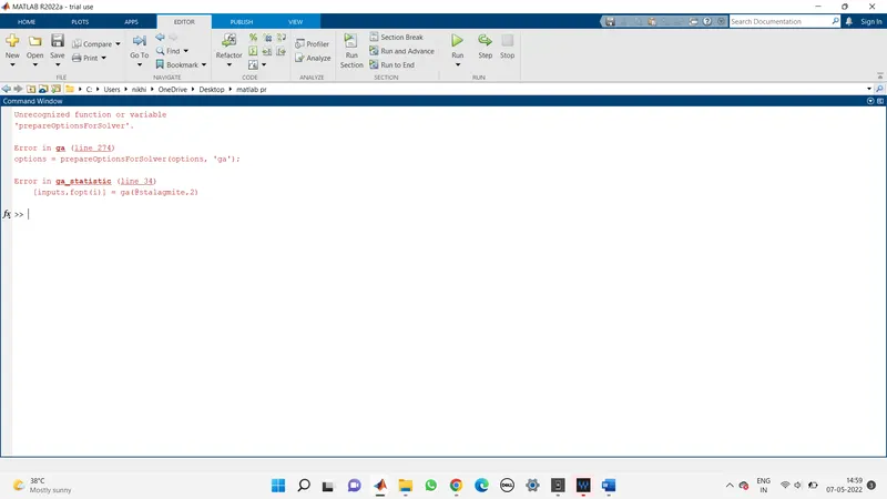
Results and Conclusions: Due to problem solver in GA our result can not come