Solving second order ODEs

Aim: Solving Second Order ODE’s using Matlab and animate the motion of the pendulum via matlab.

Objective : Pendulum have many applications . they are used in clocks and metronomes due to regularity of their period, in wrecking balls and playground swings

Explanation: First we use clear all, close all, clc. Then we put given values in problem

b = 0.05; % damping coe.

g = 9.81; % gravity (m/s^2)

l = 1; % length pf spring (m)

m = 1; % massof ball(kg) i.e. given values

Then put initial condition which is given in problem

theta_0 = [0;3]; Angular displacement is 0 and velocity is 3

Then the define time span pendulum is oscillate 0 to 20 seconds

t_span = linspace(0,20,600);

Then we use function ode

function [dtheta_dt] = ode_func(t,theta,b,g,l,m)

theta1 = theta(1)

theta2 = theta(2)

dtheta1_dt = theta2;

dtheta2_dt = -(b/m)*theta2-(g/l)*sin(theta1);

dtheta_dt = [dtheta1_dt;dtheta2_dt];

end

It is our function code that substitute in main program and also puts values of t, theta,b,g,l,m.

[t,results] = ode45(@(t,theta) ode_func(t,theta,b,g,l,m),t_span,theta_0);

Ode 45 is used solve ordinary differential equation using numerical method. In challenge there is 4rth order range kutta method . the function ode takes 3 inputs. The 3 inputs are the function to be integrated. [t , result] means that the results that have been calculated with respect to time.

Then we plot the graph i.e fig no 1 gives title is damped harmonic motion of pendulum also used lagend command for give the name of angular displacement and angular velocity.

Also label it

Then we use the for loop

Ct=1 means represent each and every frame

Then we use or put limit on x and y axis to get lines of pendulum

x_start = 0

y_start = 0

x_end = l*sin(results(i,1))

y_end = -l*cos(results(i,1))

define x and y axis

similarly for another moving line of pendulum

plot([-1 1], [0 0],'LineWidth',7)

hold on

plot([x_start x_end], [y_start y_end],'LineWidth',5)

hold on

here we plot x and y axis again with taking linewidth 7

then using markersize and markerfacecolor command we get end part of pendulum

then we use following commands to animate the movie

clear all
close all 
clc



b = 0.05; % damping coe.
g = 9.81; % gravity (m/s^2)
l = 1;  % length pf spring (m)
m = 1; % massof ball(kg)

% initial condition 
% angular dispacement is 0 and angular velocity is 5

% initial condition 
theta_0 = [0;3];

% time span 
% pendulum oscillates between 0-20 seconds

t_span = linspace(0,20,600);




% solve ODE 
[t,results] = ode45(@(t,theta) ode_func(t,theta,b,g,l,m),t_span,theta_0);

% plotting 
figure (1)
hold on
plot(t,results(:,1))
plot(t,results(:,2))
title('Damped harmonic motion of a pendulum')
legend('angular dispacement','Angular velocity')
xlabel('Time(seconds)')
ylabel('Plot')


%for loop
% before starting the loop , a counter value was defined
 ct =1;
 for i = length(results(:,1))
x_start = 0
y_start = 0
x_end = l*sin(results(i,1))
y_end = -l*cos(results(i,1))

 % plotting the animation 

figure (2) 
plot([-1 1], [0 0],'LineWidth',7)
hold on 
plot([x_start x_end], [y_start y_end],'LineWidth',5)
hold on

plot(x_end,y_end,'o','MarkerSize',30,'MarkerFaceColor','y')

title('Animation  of a pendulum')
axis([-1.5 1.5 -1.5 1]);
pause(0.03);
hold off
grid on
M(ct)=getframe(gcf);
ct = ct+1;

 end
 % Animation
movie(M)
videofile = VideoWriter('Animation of Pendulum.avi','Uncompressed AVI');
open(videofile)
writeVideo(videofile,M)
close(videofile)

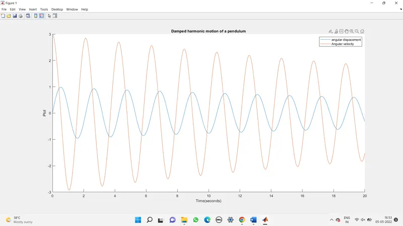
Result

https://youtu.be/vFPi9blcFfw (link for animation)

https://drive.google.com/file/d/15MG65-Yh47xsvykW8rvyQfGGuxZIg0Qc/view?usp=sharing