Cp data in curve fitting

• Aim : Write code to fit a linear and cubic polynomial for the given Cp data in curve fitting

• Objective: Curve fitting is the process to construct curve which showing difference or relation between parameter values and observed dataset. It helps to describes how your data changes mathematically.

• Explanation: First we download the Cp VS Temperature data file , then the file move in the matlab folder. First we load the file using command of load. We use comment % Preparing the data .Cp means Specific heat at constant pressure. Then we say that temperature = cp_data (: , 1) that means first column and similarly cp is second column in cp = cp_data(: , 2).

then we use plot command for plotting given data in form of graph

plot(temperature,cp,'linewidth',3);

then also give label for the axis also use the units

then we take our linear equation

%cp = A*x + B*y + C

We use polyfit command for plotting another curve

Co_effs = Polyfit(temp,cp,1)

Then we count predicted_cp

predictd_cp = polyval(co_effs,temperature);

here polyval means value of polymers and co_effs,temperature it is x and y values

Then we compare both values curve

then we take our cubic equation

%cp = A*x^3+B*x^2+c

We use polyfit command for plotting another one curve

Co_effs = Polyfit(temp,cp,3)

Then we count predicted_cp

predictd_cp = polyval(co_effs,temperature);

here polyval means value of polymers and co_effs,temperature it is x and y values

for obtain smoot curve e want to adjust value of degree

Then we compare three values of curve using commands and get the results. We got 3 different colors lines or curves which is different in color use legend command to give name of lines

clear all 
close all 
clc


% preparing the data

cp_data = load('data');
temperature = cp_data(:,1);
cp = cp_data(:,2);




%cp = Ax + By + C

co_effs = polyfit(temperature,cp,1);
predictd_cp = polyval(co_effs,temperature);





%cp =  A*x^3+B*x^2+c 

co_effs1 = polyfit(temperature,cp,3);
predictd_cp1 = polyval(co_effs1,temperature);


% Compare my curve fit with the original data

plot(temperature,cp,'linewidth',3);
hold on
plot(temperature,predictd_cp,"LineWidth",3,'Color','r')
plot(temperature,predictd_cp1,"LineWidth",3,'Color','g')
xlabel('temperature [K]');
ylabel("specific Heat [KJ/Kmol-K]");
legend('original dataset','curve fit linear','curve fit cubic')

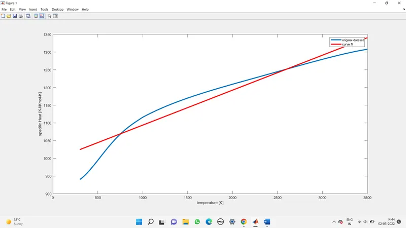
Result - Curve fit for Linear Polynomial

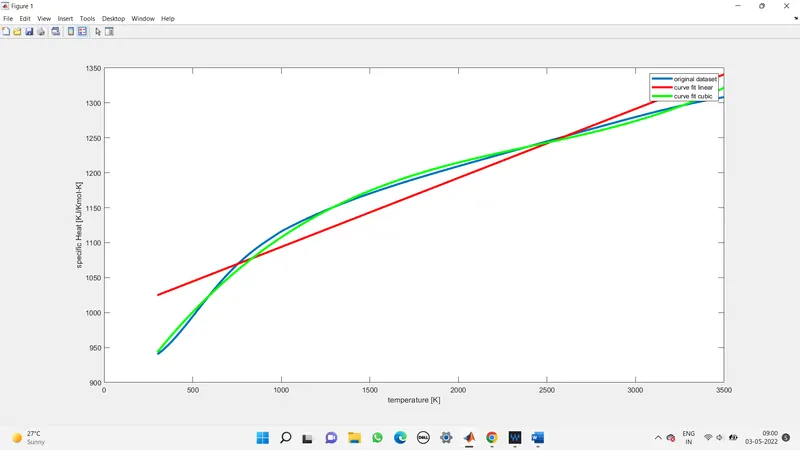
Result - curve fit for linear and cubic polynomial