Project 2 - Rankine cycle Simulator

Aim - 1. Create a Rankine cycle simulator and plot T- s and h-s diagram.

2. To Develope basic program that calculate state points.

3. To add thermodynamic relation to get points between state variables.

Theory-

Rankine cycle is process, used in power plant to produce mechanical energy from heat It usually uses water as working fluid In this cycle a fuel is used externally to convert water into steam which expands through turbine and produces work In ideal Rankine cycle pump and turbine would be isentropic, they would maximize the net work output by generating no entropy and also, we are assuming that water to steam and steam to water conversion is taking place at constant pressure.

Actual Rankine cycle differs from ideal Rankine cycle because of fluid friction causes irreversibility and heat loss to surrounding causes loss of work output pressure drops in boiler and condenser it causes, steam to leave boiler at a lower pressure.

Rankine cycle can be modified with reheat and regenerative process. Reheating cycle removes moisture carried by steam at the final stage of expansion process.it increases thermal efficiency of the cycle.in Regenerative cycle heat is exchanged between working fluid and compressed fluid before heat addition. Regenerative cycle reduces heat supplied to boiler and increases thermal efficiency

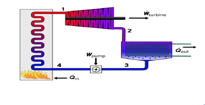
Rankine cycle

There are four processes in Rankine cycle –

1. Isentropic Expansion- Steam enters into turbine where it is expanded by turbine so pressure and temperature will decreases. Turbine generates electricity.
2. Constant Pressure Heat Rejection- The wet steam rejects heat into condenser where its phase changes again and it becomes saturated liquid.
3. Isentropic Compression- Water is pumped from low pressure to high pressure isentropically. Pump requires some input for it.
4. Constant pressure heat addition- Water enters into boiler ,where it is heated till its phase change which is dry saturated vapour. The process takes place on constant pressure and heat is added to water that’s why is called as constant pressure heat addition.

Formulas related to Rankine cycle-

heat addition = h1 - h4.

heat rejection = h2 - h3.

work done by turbine = h1 - h2.

work taken by pump = h4 - h3.

Wt-Wp

thermal efficiency=_______________

qa

net work output = Wt - wp

Wp

back work ratio (BWR) = ______

Wt

3600

specific steam consumption (SSC) =_________________

Wn

h1 = enthalpy at turbine inlet

h2= enthalpy at turbine outlet

h3 = enthalpy at pump inlet

h4 = enthalpy at pump outlet

Wt = work done by turbine

Wp= work taken by pump

(Pi,ti, hi, si) = Pressure, temperature, enthalpy, entropy at i_th state

Respectively.

clear all 
close all
clc

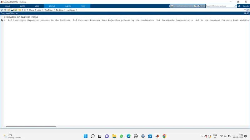
disp(  "SIMULATOR OF RANKINE CYCLE" )
fprintf('n  1-2 Isentropic Expansion process in the Turbine')
fprintf('n  2-3 Constant Pressure Heat Rejection process by the condensor')
fprintf('n  3-4 Isentropic Compression ')
fprintf('n  4-1 is the constant Pressure Heat addition Process')

% variables for stage 1
p1 = 30;
t1 = 400;
h1 = XSteam('h_pt',30,400);
s1 = XSteam('s_ph',30,h1);
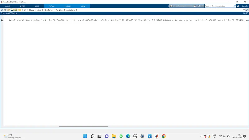
fprintf('nn       Results')
fprintf('nn AT State point 1')
fprintf('n P1 is:%f bar',p1)
fprintf('n T1 is:%f deg celcius',t1)
fprintf('n H1 is:%f KJ/Kg',h1)
fprintf('n S1 is:%f KJ/KgK',s1)


% variable at stage 2
p2 = 0.05;
s2 = s1;
t2 = XSteam('T_ps',0.05,6.1858);
sf2 = XSteam('sL_p',p2);
sg2 = XSteam('sV_p',p2);
hf2 = XSteam('hL_p',p2);
hg2 = XSteam('hv_p',p2);
x = ((s2 - sf2)/(sg2 - sf2));
h2 = hf2 + (x*(hg2 - hf2));
v2 = XSteam('v_ph',p2,h2);
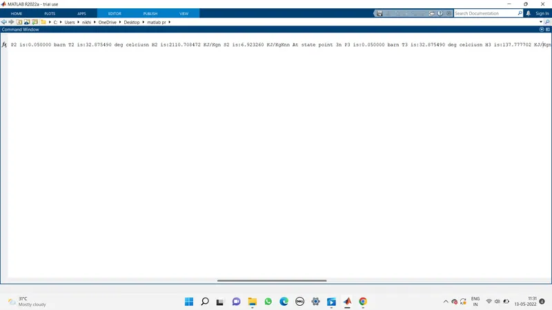
fprintf('nn At state point 2')
fprintf('n P2 is:%f bar',p2)
fprintf('n T2 is:%f deg celcius',t2)
fprintf('n H2 is:%f KJ/Kg',h2)
fprintf('n S2 is:%f KJ/KgK',s2)

% variable for stage 3
t3 = t2;
p3 = p2;
s3 = XSteam('sL_p',p3);
h3 = XSteam('hL_T',32.8785);
v3 = XSteam('v_ph',p3,h3);
fprintf('nn At state point 3')
fprintf('n P3 is:%f bar',p3)
fprintf('n T3 is:%f deg celcius',t3)
fprintf('n H3 is:%f KJ/Kg',h3)
fprintf('n S3 is:%f KJ/KgK',s3)

% variable for stage 4
s4 = s3;
v4 = v3;
p4 = p1;
h4 = XSteam('h_ps',p4,s4);
t4 = XSteam('T_hs',h4,s4);
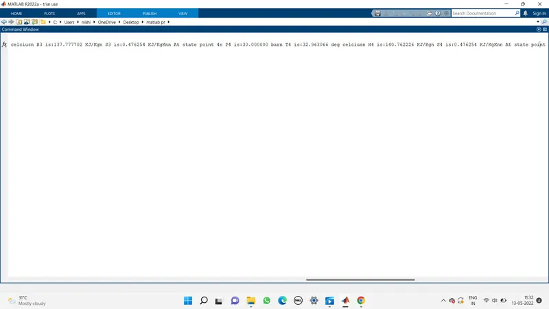
fprintf('nn At state point 4')
fprintf('n P4 is:%f bar',p4)
fprintf('n T4 is:%f deg celcius',t4)
fprintf('n H4 is:%f KJ/Kg',h4)
fprintf('n S4 is:%f KJ/KgK',s4)


% variable at stage 5
p5 = p4;
t5 = XSteam('Tsat_p',p5);
h5 = XSteam('hL_T',t5);
s5 = XSteam('sL_p',p5);
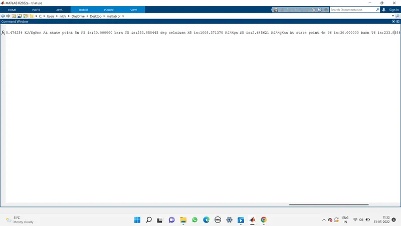
fprintf('nn At state point 5')
fprintf('n P5 is:%f bar',p5)
fprintf('n T5 is:%f deg celcius',t5)
fprintf('n H5 is:%f KJ/Kg',h5)
fprintf('n S5 is:%f KJ/KgK',s5)


% variable at stage 6
t6 = t5;
p6 = XSteam('psat_T',t5);
s6 = XSteam('sV_T',t6);
h6 = XSteam('hV_T',t6);
fprintf('nn At state point 6')
fprintf('n P6 is:%f bar',p6)
fprintf('n T6 is:%f deg celcius',t6)
fprintf('n H6 is:%f KJ/Kg',h6)
fprintf('n S6 is:%f KJ/KgK',s6)


% loop to find variables on saturated lines
t = linspace(0,400,1000);
for i=1:length(t)
    s_line1(i)=XSteam('sL_T',t(i));
end

for j=1:length(t)
    s_line2(j)=XSteam('sV_T',t(j));
end

for i=1:length(t)
    h_line1(i)=XSteam('hL_T',t(i));
end

for j=1:length(t)
    h_line2(j)=XSteam('hV_T',t(j));
end


% net work output calculation
w_turbine = h1-h2;             % work done y turbine
w_pump = h4-h3;                % work taken by pump
work = w_turbine-w_pump;       % net work output
q_in = h1-h4;                  % heat addition 
q_out = h2-h3;                 % heat rejection



%thermal efficiency 
n = work/q_in;

% back work ratio 
BWR = w_pump/w_turbine;

% specific steam consumption
ssc = 3600/work;




% plotting T-s graph
figure(1)
hold on 
plot([s_line1 s_line2],[t t])
plot([s1 s2 s3 s4 s5 s6 s1],[t1 t2 t3 t4 t5 t6 t1])
text(s1,t1,'1')
text(s2,t2,'2')
text(s3,t3,'3')
text(s4,t4,'4')
text(s5,t5,'5')
text(s6,t6,'6')
title("Rankine cycle T-s Diagram")
xlabel('Entropy(KJ/KgK)')
ylabel('Temperature(K)')
axis([0,8,0,450])

% plotting h-s graph
figure(2)
hold on 
plot([s_line1 s_line2],[h_line1 h_line2])
plot([s1 s2 s3 s4 s5 s6 s1],[h1 h2 h3 h4 h5 h6 h1])
text(s1,h1,'1')
text(s2,h2,'2')
text(s3,h3,'3')
text(s4,h4,'4')
text(s5,h5,'5')
text(s6,h6,'6')
title("Rankine cycle H-S Diagram")
xlabel('Entropy(KJ/KgK)')
ylabel('Enthalpy(KJ/Kg')
axis([0,8,0,3500])

Code Explanation -

1. first of all display - Rankine cycle simulator, using disp command.
2. Now write Rankine cycle's all process using fprintf command.
3. Assign the values of given parameters , Turbine inlet pressure(p_1) = 30 bar, Turbine inlet temperature(t_1) = 400 deg celsius,Turbine outlet pressure(p_2) = 0.05 bar.
4. Put XSteam.m file in same directory and call the XSteam function with suitable arguments to find the values of enthalpy , entropy for state 1.
5. Use fprintf command to print values of variables we found. Repeat the procedure for all other states to find unknows.
6. Now apply a for loop to find values of enthalpy and entropy at saturated temperature and store them into variables.
7. Find net work output and back work ratio with suitable formulas.
8. Plot the T-s andh-s diagram using all the value we have found in different states and give proper x and y label and add state number by text command.
9. Plot saturation line using the values we have found by for loop.

Output-

We got T-s and h-s diagram as following -

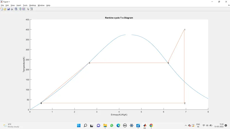
T-S Diagram

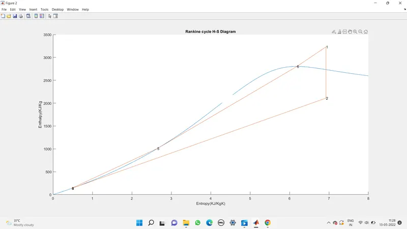
H-S Diagram

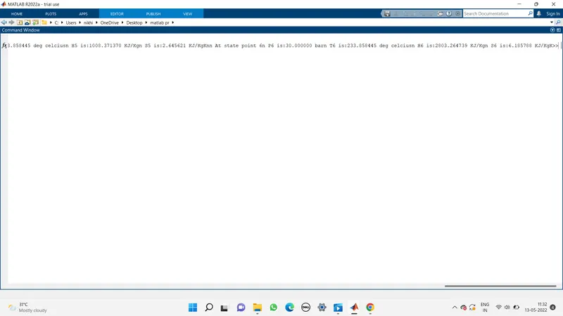
Command windows results attach Below