Final Project: Design of an Electric Vehicle

MATLAB model of the electric car which uses a battery and a DC motor

• Objectives:

  1. System-level configurations

  2. Model parameters

  3. Results

  4. Conclusion

• System-level configurations:

• The model looks like this

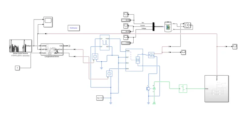
• This model represents the basic control system, controller and motor, transmission system, and battery system.

Drive Cycle Source:

• Description
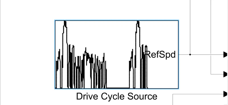
  The Drive Cycle Source block generates a standard or user-specified longitudinal drive cycle. The block output is the specified vehicle longitudinal speed, which you can use to:

  Predict the engine torque and fuel consumption that a vehicle requires to achieve desired speed and acceleration for a given gear shift reference.

  Produce realistic velocity and shift references for closed-loop acceleration and braking commands for vehicle control and plant models.

  Study, tune, and optimize vehicle control, system performance, and system robustness over multiple drive cycles.

  Identify the faults within tolerances specified by standardized tests, including:

• For the drive cycles, you can use:

  Drive cycles from predefined sources. By default, the block includes the FTP–75 drive cycle. To install additional drive cycles from a support package, see Install Drive Cycle Data. The support package has drive cycles that include the gear shift schedules, for example, JC08 and CUEDC.

  Workspace variables.

  .mat, .xls, .xlsx, or .txt files.

  Wide-open throttle (WOT) parameters, including initial and nominal reference speed, deceleration start time, and final reference speed.

  To achieve the goals listed in the table, use the specified Drive Cycle Source block parameter options.

• Longitudinal Driver:
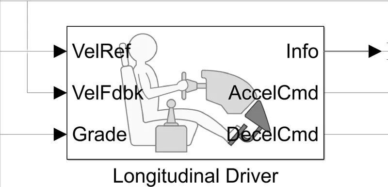
• The Longitudinal Driver block implements a longitudinal speed-tracking controller. Based on reference and feedback velocities, the block generates normalized acceleration and braking commands that can vary from 0 through 1. You can use the block to model the dynamic response of a driver or to generate the commands necessary to track a longitudinal drive cycle.
• Ports:
  Input-VelRef — Reference vehicle velocity
  scalar
  Reference velocity, vref, in m/s.
• VelFdbk — Longitudinal vehicle velocity
  scalar
  Longitudinal vehicle velocity, U, in the vehicle-fixed frame, in m/s
• Grade — Road grade angle
  scalar
  Road grade angle, θ or γ, in deg
• Output: Info — Bus signal
  bus

• Bus signal containing these block calculations.

  Signal Variable Description
  Accel yacc
  Commanded vehicle acceleration, normalized from 0 through 1

  Decel dec
  Commanded vehicle deceleration, normalized from 0 through 1

  Gear
  The integer value of commanded gear

  Clutch
  Clutch command

  Err reef
  The difference in reference vehicle speed and vehicle speed

• AccelCmd — Commanded vehicle acceleration
  scalar
  Commanded vehicle acceleration, yacc, normalized from 0 through 1.

• DecelCmd — Commanded vehicle deceleration
  scalar
  Commanded vehicle deceleration, yet, normalized from 0 through 1.

• Controlled PWM voltage:

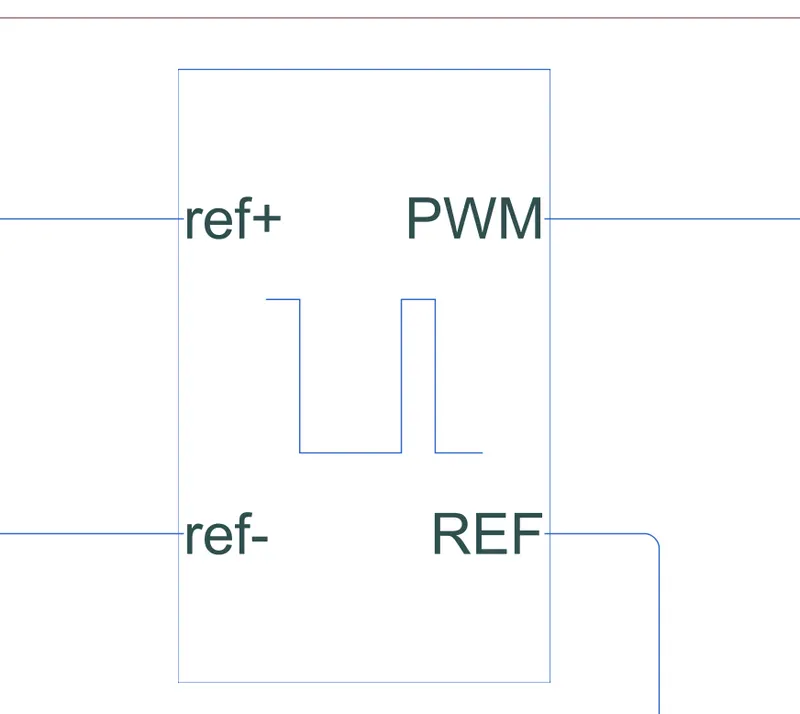
• This block creates a Pulse-Width Modulated (PWM) voltage across the PWM and REF ports. The output voltage is zero when the pulse is low and is equal to the Output voltage amplitude parameter when high. The duty cycle is set by the input value. Right-click the block and select Simscape->Block choices to switch between electrical +ref/-ref ports and PS input u to specify the input value.

• At time zero, the pulse is initialized as high unless the duty cycle is set to zero or the Pulse delay time is greater than zero.

• The Simulation mode can be set to PWM or Averaged. In PWM mode, the output is a PWM signal. In Averaged mode, the output is constant with a value equal to the averaged PWM signal.

• 

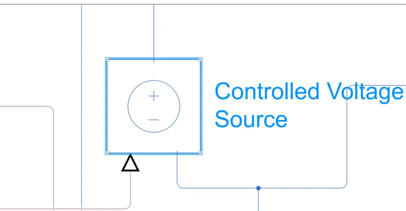
• The block represents an ideal voltage source that is powerful enough to maintain the specified voltage at its output regardless of the current passing through it. The output voltage is V = Vs, where Vs is the numerical value presented at the physical signal port.

• 

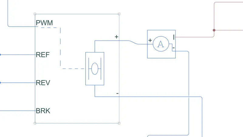
• This block represents an H-bridge motor drive. The block can be driven by the Controlled PWM Voltage block in PWM or Averaged mode.

• In PWM mode, the motor is powered if the PWM port voltage is above the Enable threshold voltage. In Averaged mode, the PWM port voltage divided by the PWM signal amplitude parameter defines the ratio of the on-time to the PWM period.

• Using this ratio and assumptions about the load, the block applies an average voltage to the load that achieves the correct average load current.

• The Simulation mode parameter value must be the same for the Controlled PWM Voltage and H-Bridge blocks.

• If the REV port voltage is greater than the Reverse threshold voltage, then the output voltage polarity is reversed. If the BRK port voltage is greater than the Braking threshold voltage, then the output terminals are short circuited via one bridge arm in series with the parallel combination of a second bridge arm and a freewheeling diode. Voltages at ports PWM, REV and BRK are defined relative to the REF port.

  DC MOTOR:

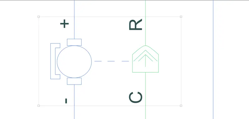
• This block represents the electrical and torque characteristics of a DC motor.

  The block assumes that no electromagnetic energy is lost, and hence the back-emf and torque constants have the same numerical value when in SI units. Motor parameters can either be specified directly, or derived from no-load speed and stall torque. If no information is available on armature inductance, this parameter can be set to some small non-zero value.

  When a positive current flows from the electrical + to - ports, a positive torque acts from the mechanical C to R ports. Motor torque direction can be changed by altering the sign of the back-emf or torque constants.

• Simple Gear

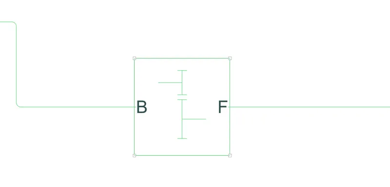
• Represents a fixed-ratio gear or gear box. No inertia or compliance is modeled in this block. You can optionally include gear meshing and viscous bearing losses.

  Connections B (base) and F (follower) are mechanical rotational conserving ports. Specify the relation between base and follower rotation directions with the Output shaft rotates parameter. Optionally include thermal effects and expose thermal conserving port H by right-clicking on the block and selecting Simscape block choices to switch between variants.

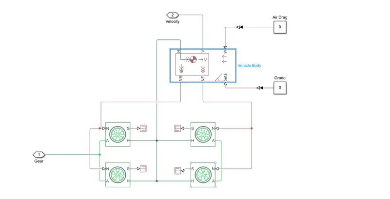
• Transmission system : This block is a subsystem containing the tires and vehicle body blocks. This block ensures the real life situations of inertia,slip of tires an velocity of the vehicle. If explored inside the transmission subsystem

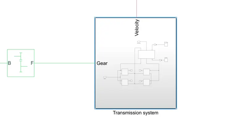
we get the below figure:

• Tire (Magic Formula):

• Represents the longitudinal behavior of a highway tire characterized by the tire Magic Formula. The block is built from Tire-Road Interaction (Magic Formula) and Simscape Foundation Library Wheel and Axle blocks. Optionally, the effects of tire inertia, stiffness, and damping can be included.

  Connection A is the mechanical rotational conserving port for the wheel axle. Connection H is the mechanical translational conserving port for the wheel hub through which the thrust developed by the tire is applied to the vehicle. Connection N is a physical signal input port that applies the normal force acting on the tire. The force is considered positive if it acts downwards. Connection S is a physical signal output port that reports the tire slip. Optionally expose physical signal port M by setting Parameterize by to Physical signal Magic Formula coefficients. Physical signal port M accepts a four element vector corresponding to the B, C, D, and E Magic Formula coefficients.

Vehicle body:

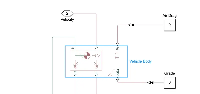
• Represents a two-axle vehicle body in longitudinal motion. The block accounts for body mass, aerodynamic drag, road incline, and weight distribution between axles due to acceleration and road profile. The vehicle can have the same or a different number of wheels on each axle. Optionally include pitch and suspension dynamics or additional variable mass and inertia. The vehicle does not move vertically relative to the ground.

• Represents a two-axle vehicle body in longitudinal motion. The block accounts for body mass, aerodynamic drag, road incline, and weight distribution between axles due to acceleration and road profile. The vehicle can have the same or a different number of wheels on each axle. Optionally include pitch and suspension dynamics or additional variable mass and inertia. The vehicle does not move vertically relative to the ground.

Battery:

• Implements a generic battery model for most popular battery types. Temperature and aging (due to cycling) effects can be specified for Lithium-Ion battery type.

• 
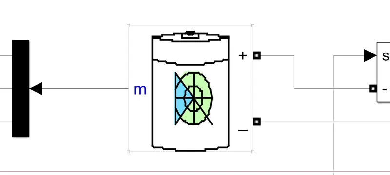
• The above model is a battery system for measuring the SOC,current,and voltage of the vehicle design. The other battery model can be used just for discharging and not charging. Here as we use both Acceleration and braking command of the motor , voltae from the battery needs to be both discharged and charged back while regenerative braking.

The Drive cycle source provides the reference drive cycle as per requirement. The longitudinal block takes it as ana input for vehicle reference speed and compares it with actual velocity of the vehicle for accurate analysis. The output of longitudinal driver block is info,accelerator command and decclerator command. We do not want the info terminal so connect it to a terminator. The accelerator command is given to the 'controlled pwm voltage' block. By default it is set to pwm mode so change it to average mode. The output frequency is also changed to 10000 Hz from 1000Hz. The H-bridge is connected between the 'pwm' and 'ref' terminals of the 'controlled pwm source' block. The 'BRK' terminal of the H-Bridge is connected to the decelerator command form the longitudinal driver respectively.

---------------------------------------------------------------------------------------------------------------------------------------------

• The following results were obtained for default values of Grade,Output Voltage ,Output Current and SOC of battery , Air Drag of vehicle body:

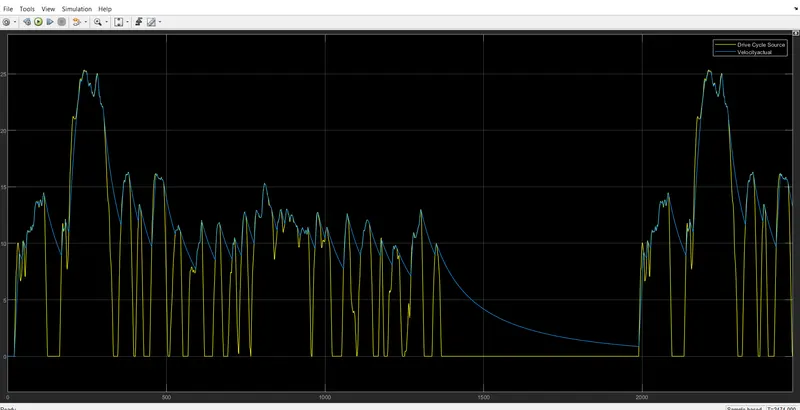
From the above figure it is evident that the Drive cycle and the actual velocity tend to be equal for some instances and the drive cycle falls to zero but actual velocity is close to zero but not equal to zero. This could be because the vehicle for drive cycle recording would be different than the desired EV here. But the model tries to replicate as much as possible which is a desirable aspect. The actual velocity is a feed back from the output velocity from the transmisssion system. The Drive cycle is the reference velocity. For some of the time the vehicle is seen to be at rest until for one more time at nearly 2000 seoconds the vehicle runs for one more time. The velocity of the vehicle at t=0 is 0 but seen steeply increasing for 15 kmph. Again it inceases the speed and increases to 25 kmph. Maximum peaks can be seen for 10mph and 15 kmph. Just 2 peaks are seen for 25 kmph.

Battery parameters:

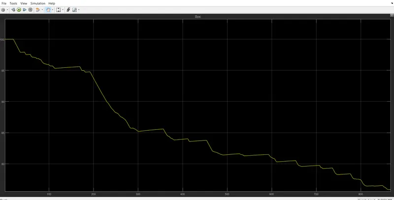
1-SOC(state of charge) - The state of charge shows the amount of charge present in the battery for the given instance of time. As seen above the state of charge is initially 100%. After starting the vehicle the SOC starts falling down for the initial 100 seconds. An important aspect for an efficient design should be that whether or not the battery is recharging during the braking operation alongwith proper discharge of the battery. From the characteristics the spikes rising back show recharging and the downward decrease show discharging accordingly.

2- Current-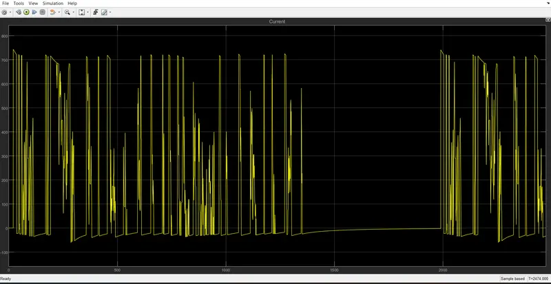

The current spikes are seen analogous to the drive cycle to some extent. This is a graph showing Output current in amps v/s time in seconds. The points wherever the current shows up to its peak value is almost near to 700 amps. The current is consumed by the motor via the controller which is the H-bridge here. An efficient vehicle needs to have peak current consumption periods to be lowest so as to prevent the windings from burning. In this case it is seen to be fulfilling this criteria.Even is the vehicle is running at a uniform speed does not mean that the current could be also constant and could be affected by other parameters of motor design.

3-Voltage

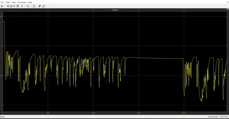
The voltage at initial level :

The initial voltage across the battery is near about to 8.5V. As the vehicle starts the voltage level falls down to 7.5 and again the spikes similar to that of the drive cycle are seen apparently.When the vehicle is at rest the voltage is a straight line between 7.5 & 8.5 V. The conjusted yellow graphs suggest there is variation in voltage and voltage demand is high. The lowest voltage seen is near to 7.1V when the vehicle is stopped or deceleration is applied.

The actual velocity directly noted from the vehicle body is same as that of the feedback velocity.

Comparison of different drive cycles:

Drive Cycle	FTP75 urban	FTP75 Highway	US-06	ECE-1	New YOrk City
Maximum speed (kmph)	86.4	97.7	128.5	120	44.6
Average speed(Kmph)	27.9	79.3	77.5	49.9	12.2
Total Traction energy (kWh)	10.47	10.45	17.03	11.79	15.51
Drag(kWh)	5.95	9.47	11.73	8.74	4.69
Total Enrgy consumed by braking(kWh)	4.52	0.98	5.30	3.05	10.82
Percentage of braking energy to total traction enrgy(%)	43.17	9.38	31.12	25.87	69.76

The above tests indicate a 1000 kg mass vehicle travelling for 100 km for diffenrent drive cycles. FTP-75 is of 2 types - highway and urban. The highway drive cycle is seen to be more efficient as there are ideal conditions for driving such as longer high speed durations,limited braking instances and rollin resistance. The total energy consumes by braking for FTP-75 urban is 4.52 kW whereas it is 0.98 for FTP urban. ECE-1 is not a real life drive cycle but just designed for lab conditions.

• DC-Motor specifications:
• Field type-Permanent Magnet
• Model parameterization- By rated load and speed
• Armature inductance-12 uH
• No-Load speed-19100 rpm
• Rated speed (at Rated load)-15000 rpm
• Rated load (mechanical power)- 50000 W
• Rated DC supply voltage- 300V
• Rotor damping parametrization- By damping value.

Here for obtaining the increased torque the rated load was changed to 50kW and rated DC supply voltage was changed to 300v .

parameters could be varied for testing the conditions.