Week 7 State of charge estimation

The Battery model:

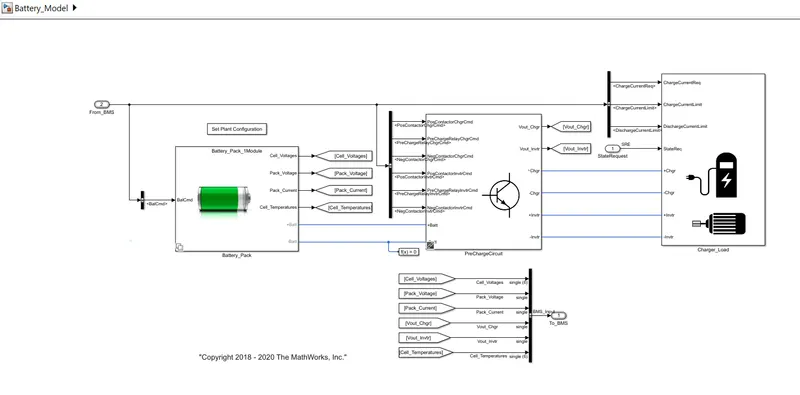
In this model, the input is taken from the Input port named "from_BMS".It is then fed to three block sets simultaneously. The three Blocks are Battery pack, PreChragerCircuit, Charge Load. To set the configuration click on set plant configuration and choose one from the two options. Here the option chosen is battery pack 1. The output from this block is 1-Cell voltages,2-Pack Voltages,3-Pack Current,4-Cell Temperature.

The next block is Pre charger circuit which takes the input from the BMS and via Bus-selector block extracts or splits the signals into respective components. This is done by the Data-Conversion Block

Convert the input to the data type and scaling of the output. The conversion has two possible goals. One goal is to have the Real World Values of the input and the output be equal. The other goal is to have the Stored Integer Values of the input and the output be equal. Overflows and quantization errors can prevent the goal from being fully achieved. The components or the inputs given to the Pre-Charger circuit are :

1. Positive contactor charger command
2. Pre-charge Relay charger command
3. Negative contactor charger command
4. Positive contactor inverter command
5. Pre-charge relay inverter command
6. Negative contactor inverter command

The next block is : Charger Load whose inputs are Charge current requirement, Charge current limit, Discharge current Limit.

If you double click on the same block the following block appears:

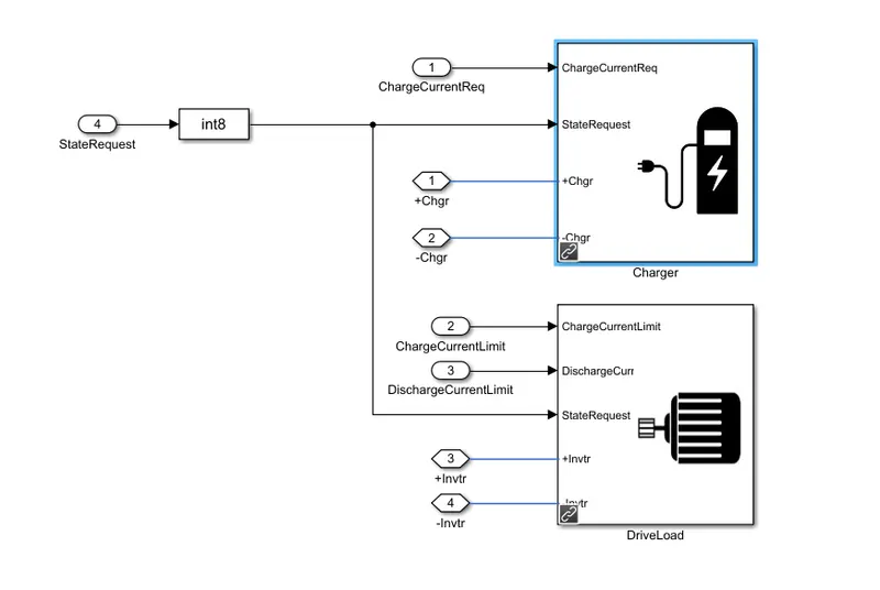
The output here is taken from Inverter + and Inverter - , Charger+ and Charger - terminal with initial data-type conversion for converting to int8 type.

The next model is : BMS closed loop

The input taken is just one : state request . The corresponding outputs given are : BMS input, BMS output and BMS Info . The feedback is given to the ECU block via unit delay block for Sample and hold with one sample period delay.

The final model is BMS_closed_loop_test_harness_dashboard .From this dashboard choose the serial number of the test case which you want to simulate.

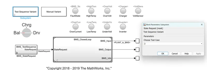
In this image, the test case selected is test case number 3. After starting the simulation the graphs are shown like this:

Test Case 1:

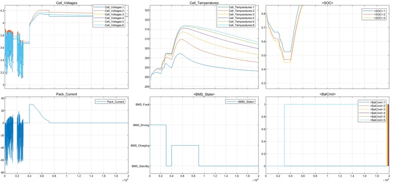
For test case number 1, the Cell voltages are fluctuating for 1/4 th of the starting time and later on rises gradually and finally at 4.2 volts it stabilizes uptil the end of the simulation time. The cell temperature for cell number 5 is lowest starting at 200 and it increases with decrease in cell number i.e for cell number 1 the temperature is the highest at around 310. The SOC graph is showing all the three SOC of the three individual cells. SOC of the cell 1 is the highest throughout the cycle and SOC of the cell 3 is the lowest throughout the simulation. Talking about the Pack current , the starting of the simulation is totally pure spikes which shows instability of the system. The BMS state shows three conditions : BMS_Driving, BMS_charging,BMS_standby

The extra state BMS_fault is present to show if any fault has occurred.

Test 2:

For test case 2 all the parameters appear to be identical to test case 1. So not a very significant variation is seen in comparison.

Test3:

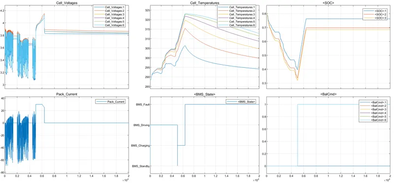
Test case 3 has different output characteristics than 1 and 2. Talking about cell voltages they are for 0.4-time units the fluctuation is seen clearly. Then after a small spike all the voltages stabilize at around 3.8V. The cell temperature pattern is similar to test case 1 and test case 2. The SOC pattern is also similar to other test cases except here the stabilized SOC is seen. Here BMS state is showing fault and BMS driving,BMS charging and BMS standby. The balance command is provided for cell 1.

SOC estimation model-ECU block

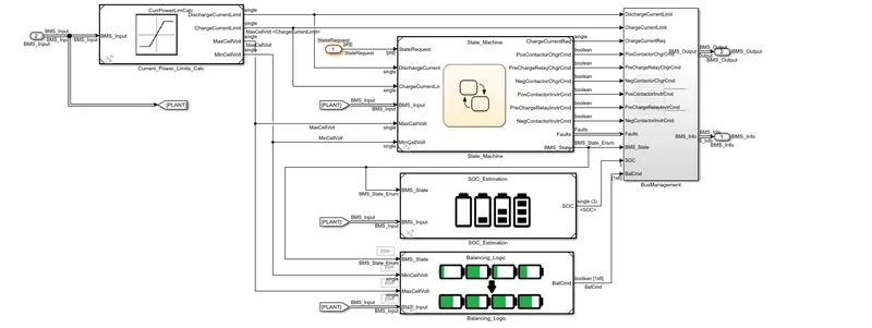
The first block is the saturation block and other inputs given to state machine are PLANT, STATE REQUEST, Max cell voltage. The two blocks below the state machine are SOC_estimation and Balancing logic blocks. The outputs are given to the subsystem Bus management. The outputs are :

1. Discharge current limit
2. Charge current limit
3. Charge current req
4. PosContactor Charge command
5. Pre charge relay charger command
6. Negative contactor charger command
7. Positive contactor Inverter command
8. Pre charge relay inverter command
9. Negative contactor Inverter command
10. Faults
11. BMS_State
12. SOC
13. Balance CMD

State machine

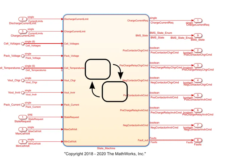
State machine>>State machine

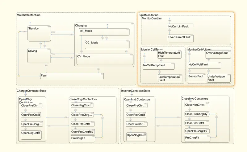
The above image shows the logical state transitions for the overall model. The different state machines are Main state machine, fault monitoring, charger contactor state, Inverter contactor state. Each state by default will try to constantly change the current state.

In this way the coulomb counting method is implemented.