Project - Position control of mass spring damper system

Differential equations represent the dynamic behaviour of the physical systems.

• Newton's Second Law states that "an applied force is proportional to the rate of change of momentum.
• Mathematically: `F alpha d/dt(m*v) or F = m*d/dt(v) or F=m*a`
• where:
• 'F' is the applied force
• 'm' is the mass and the proportionality constant.
• 'v' is the velocity
• 'a' is acceleration

• If 'X' represents the displacement , 'xdot' represents the velocity , and 'xdotdot' represents the acceleration then the above equation can be written as :
• F=m*a = m*xdotdot
• Here the dot represents the time derivative.
• In reality , dynamic systems should consider the damping manifested by the medium operating with its associated stiffness.
• With these two additional terms, the governing differential equation can be written as
• F(t) = m*xdotdot + c*xdot + k*x
• where 'c' is the damping coefficient, and 'k' is the stiffness constant
• Both 'F' and 'x' are functions of time.

• Differential equations in this form are suitable to represent the mechanical systems that are termed as "spring-mass-damper" systems.
• In Matlab and Simulink, the differential equations are covered into algebraic equations by using the 'Laplace transforms'
• The Laplace transform of a function is defined as :
• `L[f(t)] = F(S) = int_0^oo f(t)*e^(st)dt`
• When we apply Laplace transform to the differential equation that was previously discussed i.e. , f(t) = m*xdotdot + c*xdot + k*x, we obtain:
• F(S) = m*S^2X(s) + c*s*x(s) + k*x(s) or (m*s^2 + c*s + k)*x(s)
• Where 'S' is the Laplace Variable
• 'F(s)' is the Laplace transform of f(t)
• 'X(s)' is the Laplace transform of x(t)
• 'Laplace transform' conversion ignores the initial conditions and
• X(s)/F(s) = 1/ (m*s^2 + c*s +k)
• This is called the transfer function.
• It is easier to simplify the transfer functions using the block

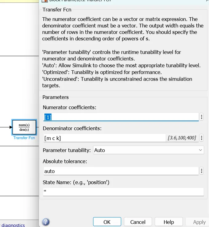
Transfer function of mass-damper is : 1/(m*s^2 + C*s + k)

The "Inverse Laplace Transform" is applied to these individual fractions will yield the solution in the time domain.

• "Laplace domain" is treated as a frequency domain.
• f(t) = m*xdotdot + c*xdot + k*x
• The forcing function , f(t) is also known as the input.
• f(t) can take the form of any function (step, ramp, pulse , signal builder) to mimic a physical situation.
• When f(t) is 0 , the response is called an initial condition response.
• When f(t) is non-zero, the response is called a forced response.
• We have defined the differential equation with the coefficients m,c and k that represents mass, damping coefficient, and the stiffness constant of the mechanical system under consideration, respectively.
• It is called a Spring - mass - damper system as mentioned earlier.
• The characteristics of such systems systems are dependent on the parameters m,c and k.

• The natural frequency of the dynamic system wn can be defined as wn = sqrt k/m.
• Where wn is the natural frequency of the dynamic system.
• The natural frequency determines the frequency determines the frequency at which it oscillates.
• This happens

• When the dynamic system is subjected to a forcing function (like an impulse acting for a very short duration with a large magnitude).
• When the dynamic system is not subjected to any restraining forces like damping.
• On the other hand , when the dynamic system is subjected to a sustaining force with the same frequency of the dynamic system , the resonance phenomenon occurs , and this causes system failure.
• The damping coefficient , c , can be defined
• 2*`zeta*omega = c/m`
• Where `zeta`is the damping ratio and
• wd = wn*`sqrt (1- zeta^2)`
• Where wd is the damped frequency

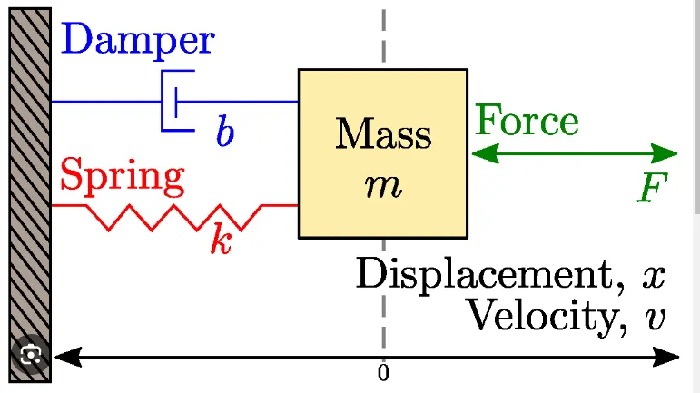
• If a forcing function , f(t) is applied to compress the spring or extend the spring and when f(t) is released the dynamic system will exhibit simple Harmonic motion with the governing differential equation :
• m*d^2x/dt^2 + k*x = 0 (Or) m*d^2x/dt^2 = - k*x

Control System Design :

• Control systems find applications in a variety of industries , including Aerospace, Automotive , Electrical, Mechanical, Electronics and chemical.
• In all these applications , a dynamic system is controlled in such a way that its output is regulated around a set point or made to track a commanded input.

The parameters provided are as follows:

1. m = 3.6 Kg
2. k=400 N/m
3. c=100 Ns/m

The Script file for loading these parameters into Workspace is as follows:

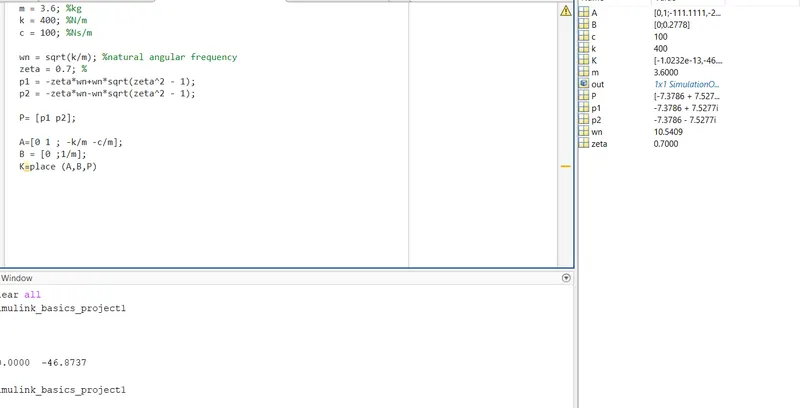
The poles are found and using the PLACE command the coefficients Kp/K(1) and Kd/K(2) are computed. So the governing input for the model is the damping factor 'zeta' , which is undamped here.

The corresponding model for the above parameters is as shown below:

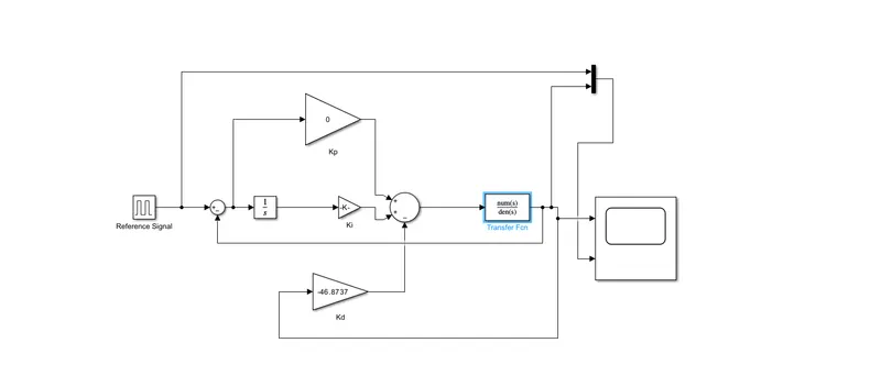
The reference signal is used from the pulse generator which has the parameters as shown below:

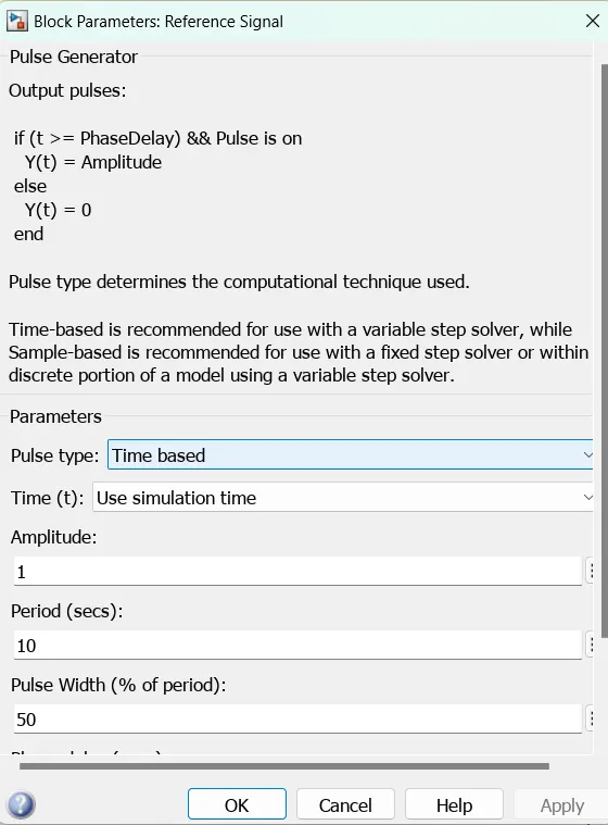
pulse width is 50% and time period is taken as 10 seconds so T (on) = 5 s and T (off) = 5s. Amplitude is taken as unity.

• Definition of time domain characteristics:

1. Rise time (Tr) : The time required for the response to rise from 10% of the final value to 90 % of the final value.
2. Settling time (Ts) : The Time required for the output to settle within a certain percent of its final value and is specified in terms of the time constant (T); Where τ=1ζ⋅ωn�=1�⋅��and a typical settling time i chosen as : Ts = 4 / (ζ⋅ωn)(�⋅��).
3. Overshoot : The maximum deviation or excursion of the response above the steady state value.
4. Steady State Error (Ess) : The hang-off error between the desired steady state value and the actual steady state value.

• Control Design Objectives
• Settling time < 2s
• Overshoot < 5%
• Steady state error < 1%

1. For Ki = 176

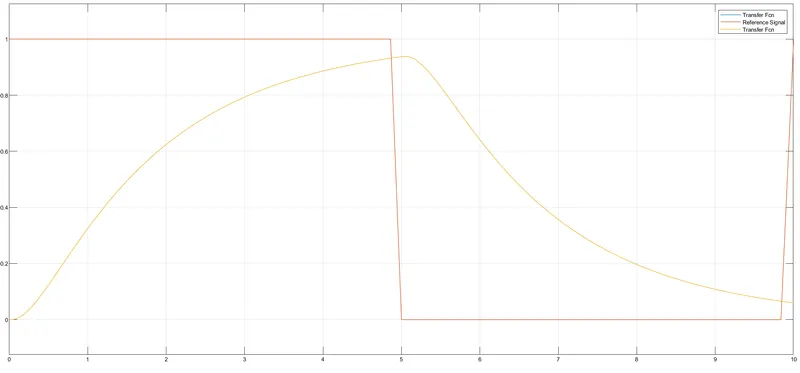
The PID control system for mass spring damper system is seen to be clearly violating the time domain characteristics / Control Design Objectives

2. For K = 1000

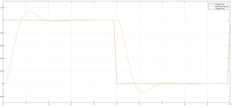
The PID Control system for mass spring damper system is showing a slight overshoot about around 1.15 units . Which is still not as per the Control Design Objectives.

3. For Ki = 650

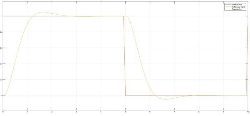
The Overshoot is decreased significantly and seen to be tracking the reference signal.

So the Control Design Objectives are seen to be satisfied as compared to the above two cases. Hence the System is tracking the reference signal successfully.