Final Project: Electric Rickshaw modelling
Aim: To create a detailed MATLAB model of an electric rickshaw.
Objectives:
- Rear wheels driven by PM brushed type motor.
- For any three standard driving cycles show energy consumption.
- For any three standard driving cycles show the temperature rise of the motor and controller for 100 km constant speed driving at 45 kmph.
Abstract:
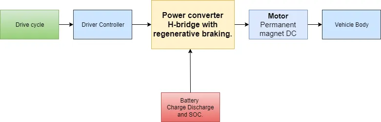
- Here the EV model used comprises of the components as shown in the block diagram below. The adaptation of EVs is becoming key performance indicator for the efficient functioning of the economy with the major reason being inflated prices of crude oil and consequently petrol and diesel.
- Although EVs are not the only convenient option being considered but there are many useful things that make a person to switch from fossil fuel dependency to clean energy based transport. E-rickshaw is one of types of EV. Usually the three wheeler EV allows 4 - 5 people as load and 48 v battery alongwith 1KW DC motor which is almost completely BLDC most of the times. But still three wheeler EVs are not suggested by the company itself for operating in the extreme terrains like mountaineous regions or slopes.
Block diagram:
- First we have a vehicle body and the dc motor is connected to the axle of the wheels. Before connecting the battery directly to the motor we require a motor controller. This motor controller is nothing but the device used for deciding at what speed the motor should be run to obtain the desired speed.There is a drive cycle input and there is a driver controller input which will actually track the speed of the verhicle and which will match with the given input.
Tire
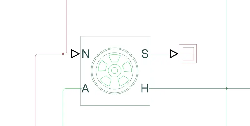
We need to model three wheeler so we need to have 3 such tires. So one tire is on front axle and two wheels are on the rear axle. We are going to connect the shaft of the motor to the transmission system through the rear axle. There are four terinals to this H stands for the Hub, S is the tire sleep N is the normal force which is applied to the tire A is the axle connection. These are the four terminals of the wheel block.
Now we are going to connect the vehicle body which is going to be actually mounted on the wheels of the vehicle.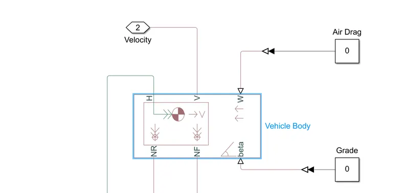
The wheels are connected to the vehicle. To do this we need to connect the hub of the vehicle to the hub of the wheel.
If we open this blocks there are parameters available according to individual tires. Choice is available from peak longitudinal forces and slip and other options. Apart from that rolling resistence and damping coefficient can be selected. On double clicking the vehicle body, the block parameters are seen. The vehicle body weight is seen which is 1200Kg, number of wheels on axle is 2. The frontal area in m2 is shown. You can enter the drag coefficients and you can have the pitch related dynamic as well. With this vehicle body configuration you now need to connect various ports to this block. The axle of the two tires is connected with the gear system. A simple gear is used.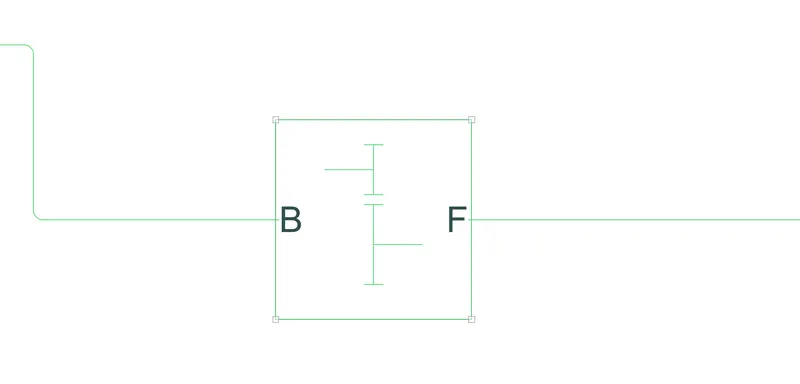
The output of this part is connected to gearbox. There will be some input coming from the shaft of the motor which will be connected to this gearbox.
The rear axle is connected with the motor. We need to connect the front axle of the front wheel and the noral force is needed to be applied on the rear part which is 'Nr' connected to N of the wheels on the rear axle.
Here is one popular model I found on the internet. It is designed by the company https://www.gemev.com/prince-e-rickshaw.html
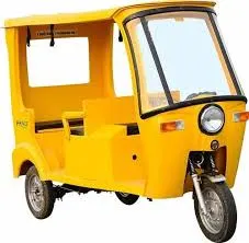
Special Features Prince
- Increased rear shocker performance
- Wider seating Space
- Option for rear glass and other accessories
- A lot of space for advertisement
- Warranty on most parts
- High storing capacity
- Light in Weight
- Better range per charge than any other E Rickshaw
- FRP Lasting much longer
- Easy to Repair FRP in case of accidental damage
Technical Specifications Prince
| Features: | Specifications: |
| Seating Capacity | 4P + D |
| Dimensions - Length*Width*Height - mm | 2758mm * 998mm * 1770mm |
| Dimension (Back Panel) - mm | NA |
| Wheel Size | 3“x12”, 6PR |
| Vehicle Kerb Weight - Kg | 282Kg |
| Gross Vehicle Weight | 682Kg |
| Top Speed | 25 kmph |
| Motor Power | 1kW |
| Motor Type | BLDC Motor |
| Battery Type | Lead Acid / Li-Ion |
| Battery Capacity | 70 Ah - 110 Ah |
| Range | 80KM - 120 KM |
| Charger | 48V, CCCV-SMPS |
| Transmission Type | Direct Drive |
| Suspension(Front & Rear) | Telescopic shock absorber & Leaf Spring |
| Brakes | Mechanical Drum brake |
| Maximum Braking Distance | 2m |
| Roof Type | Hard Top |
Now we need to plot the efficiency of the vehicle for 3 standard drive-cycles and one for constant 45 kmph speed for 100 kms.
1.Outputs for constant signal:
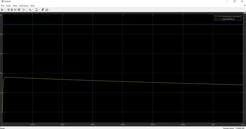
- Input vs output velocity:
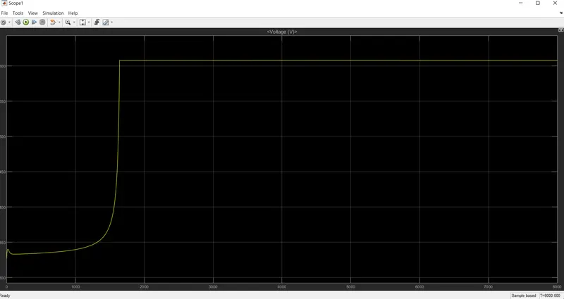
- Battery Voltage:
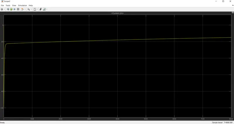
- Battery current:
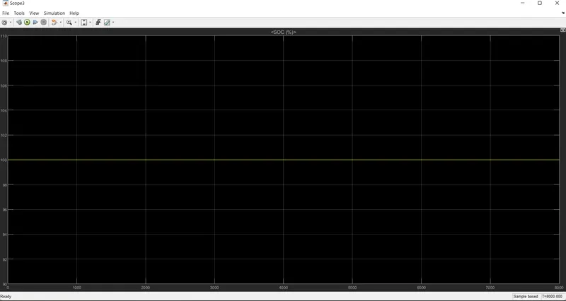
- Battery SOC:
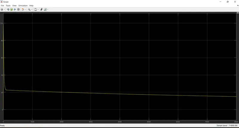
- Motor current:
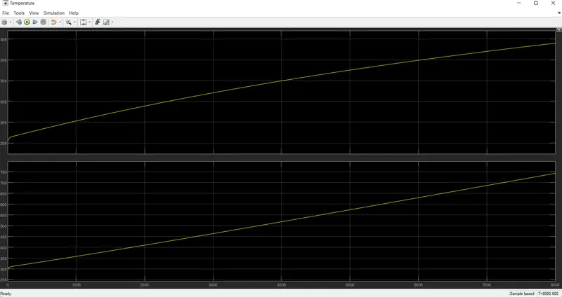
- Motor temperature and H-bridge temperature:
- In this condition the vehicle is moving at a constant speed 45 kmph for distance 100km. So motor current remains constant, Battery SOC is also constant because no significant change is seen in motor current and whatever the rise is observed, it is of a gradual slope.
- But the temperature of the motor keeps increasing and reaches at 308 k which was 298 k at the initial condition.
- Same identical pattern is observed for H-bridge temperature variance. So this is not a desirable scenario but this is an imaginary condition because in most cases the vehicle speed cannot remain accurate and acceleration and deceleration is always observed in practical cases.
The next drive cycle is chosen as HWFET:
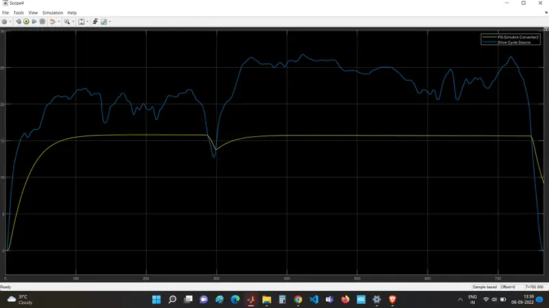
- Input vs output velocity:
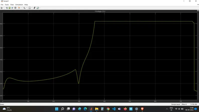
- Battery voltage:
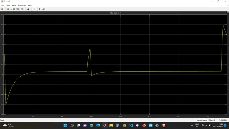
- Battery current:
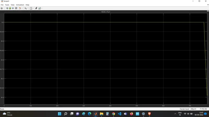
- Battery SOC:
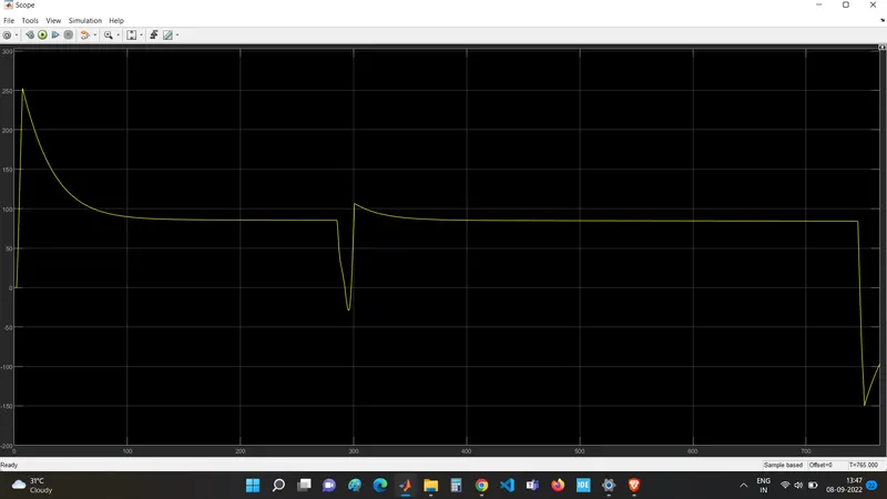
- Motor current:
- Motor temperature and H-Bridge temperature:
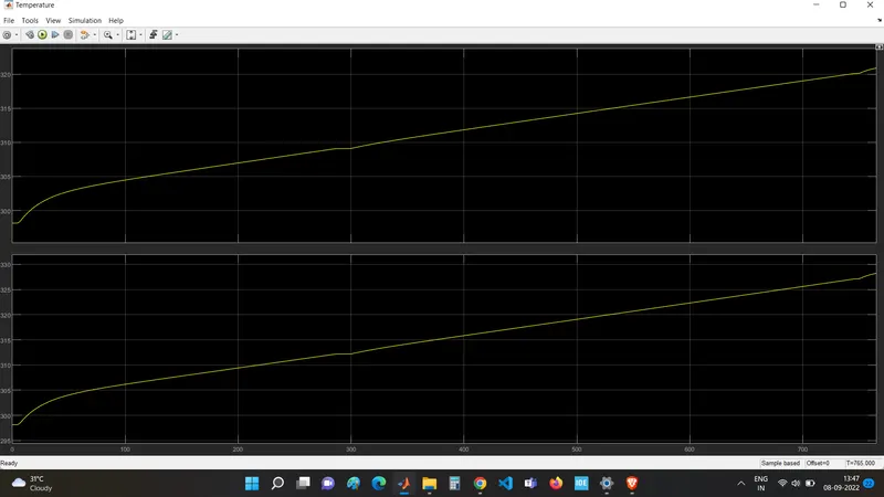
- Here firstly by seeing the scope for input vs output velocity , it is evident that the vehicle is not able to track down and follow the same pattern as that of input but it is still close to the pattern and also the uniform velocity is seen at the output. The battery voltage shows rapid variation with respect to battery current. The temperature of the motor and H-Bridge is seen rising more than that of the previous case. Battery SOC is Constant throughout the drive cycle except at the ending it falls to 99.6%.
2.Output for FTP-72 drive cycle:
- Input vs output velocity:
- Battery voltage:
- Battery current:
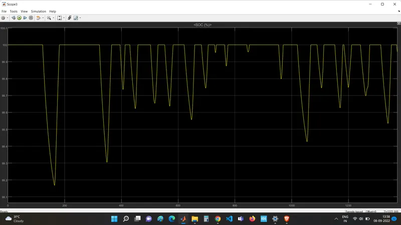
- Battery SOC:
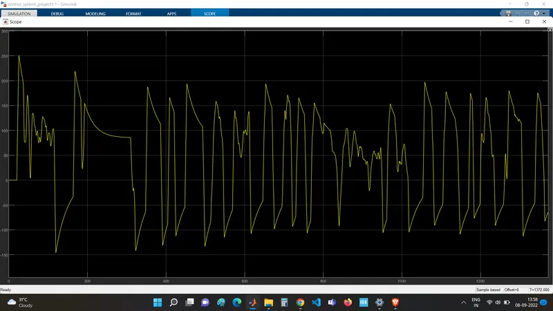
- Motor Current:
- Motor temperature and H-Bridge tempearture:
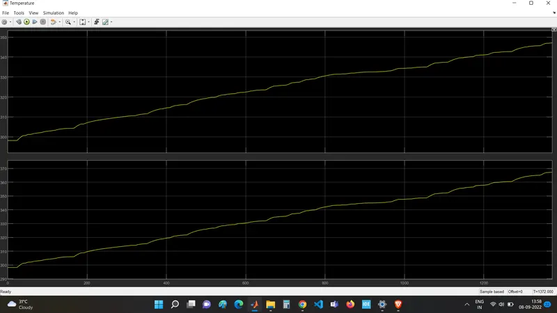
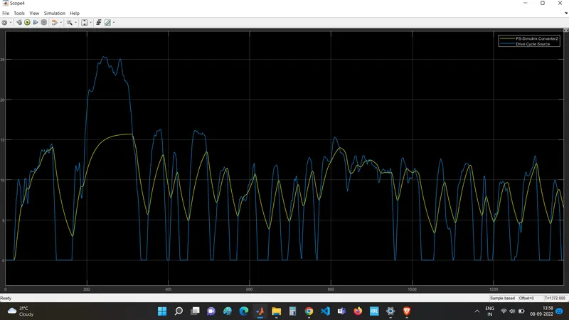
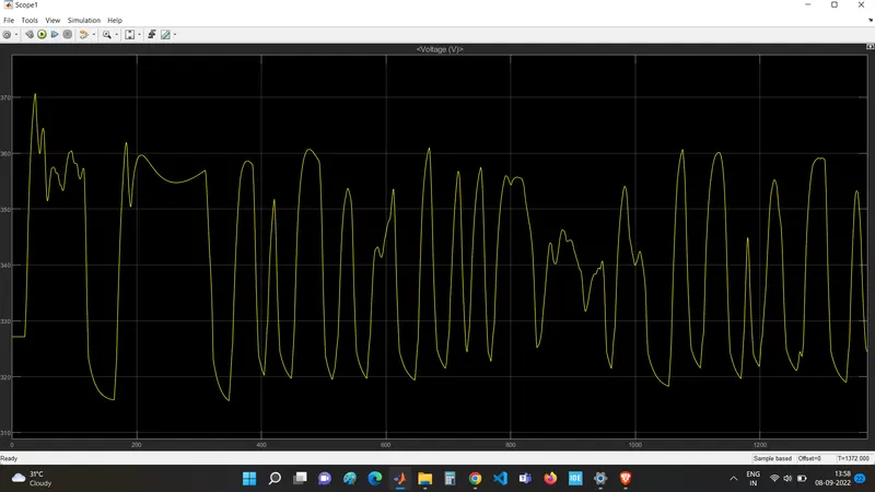
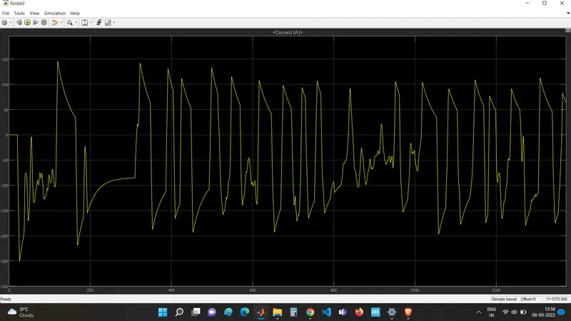
- Now the notable change observed here is that with an increase in Drive-cycle time, the accuracy of the reference tracking aspect increases. Here the temperature is more than previous 2 drive cycles. The motor current, battery current are identical and battery voltage is also seen with increase and decrease with non-uniform slope.
3.Output parameters for LA92 drive cycle(1435 seconds):
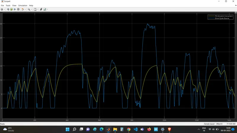
- Input Vs Output velocities:
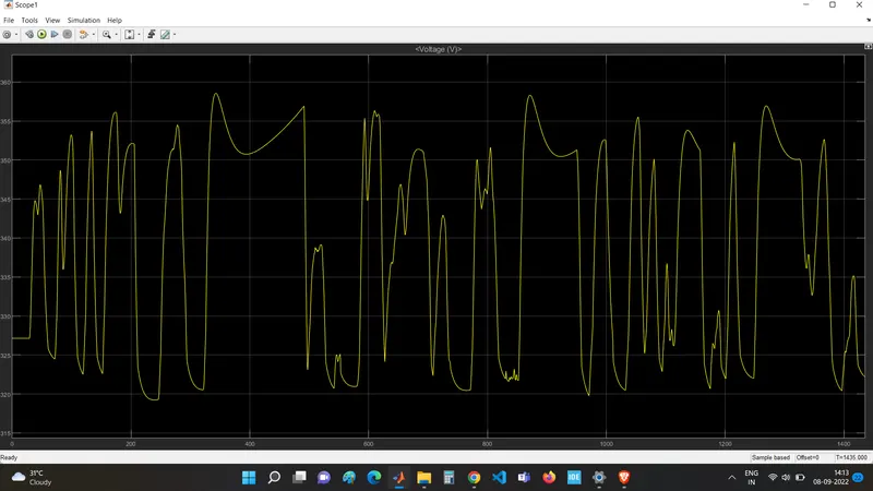
- Battery Voltage:
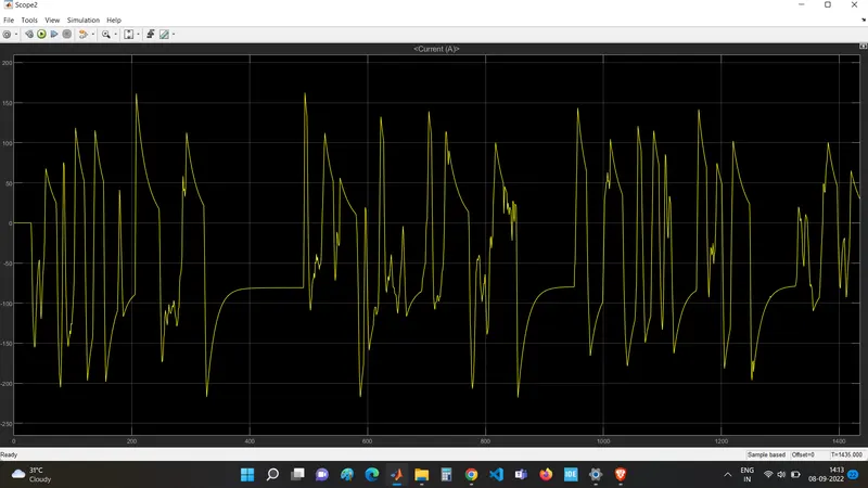
- Battery Current:
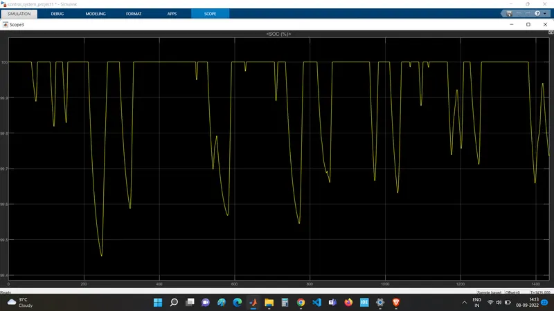
- Battery SOC:
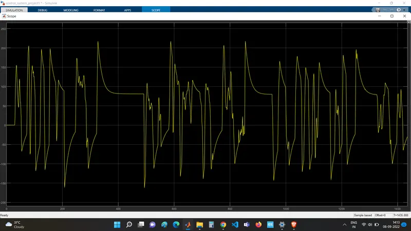
- Motor current:
- Motor and H-Bridge temperature:
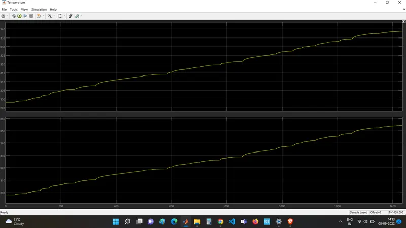
- Here also the vehicle is unable to track the accurate points of the drive cycle. The spikes are seen in motor current and battery current indicating motor operating in full-load region.Here the temperature is again above 340 K. The battery SOC is also seen varying according to pattern of drive cycle:
- In all the above cases wherever there are spikes in the scope, they can be removed by increasing the mechanical power of the motor and voltage of the battery.
The parameters for motor are:
| Feature: |
Specification: |
|
Field type : |
Permanent Magnet |
|
Model parameterization |
By rated load and speed. |
| Armature Inductance | 12 micro H |
|
No-load speed: |
3000 rpm |
|
Rated speed (at rated load): |
2500 rpm |
|
Rated load (mechanical power): |
4 KW |
|
Rated DC supply voltage: |
60 V |
|
Rotor damping parameterization: |
By damping value |
The parameters for vehicle body are:
| Feature | Specification |
|
Mass: |
659 Kg |
| Number of wheels per axle: | 2 |
| Horizontal distance to CG from front axle: | 1.4 m |
| Horizontal distance from rear axle: | 1.6 m |
|
CG height above ground |
0.5 m |
|
Frontal area: |
3 m^2 |
|
Drag coeffiecient |
0.4 |
|
Air-density: |
1.18 Kg/m^3 |
The parameters for H-bridge are:
| Features: | Specification: |
|
Power supply: |
Internal |
| Simulation Mode: | averaged |
| Regenerative braking : | Always enabled braking for linearization. |
| Load current characteristics: | Smoothed |
|
Enable threshold voltage: |
2.5 V |
|
PWM signal amplitude: |
5.0 V |
|
Reverse threshold voltage: |
2.5 V |
|
Braking threshold voltage: |
2.5 V |
|
Output voltage amplitude: |
60 V |
|
Total bridge on resistance: |
0.1 Ohm |
|
Freewheeling diode on resistance. |
0.05 ohm |
|
Measurement temperature: |
298.15 K |