Final Project: Design of an Electric Vehicle

AIM:-

Create a MATLAB model of an electric car that uses a battery and a DC motor. Choose suitable blocks from the Powertrain block set. Prepare a report about your model including the following:

Objectives:

1. System-level configurations

2. Model parameters

3. Results

4. Conclusion

ANSWER:-

Types of Electric Cars and Working:-

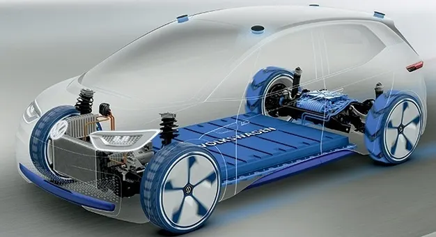
Different types of electric cars changed and are developed continuously giving users and potential users choices. Today the world is increasingly familiar with the terms BEV, HEV, PHEV, and FCEV. How does an electric car work? How an electric vehicle works is depending on the type. This article will briefly discuss the types and working principles of electric cars or vehicles marketed in the World and Indonesia today.

An electric car is a vehicle that is fully or partially propelled by electric motors, using energy stored in rechargeable batteries. The first practical electric cars were produced in the 1880s. Electric cars were popular in the late 19th century and early 20th century. Innovation and advanced development in internal combustion engines (ICE) and mass production of cheaper gasoline vehicles have led to a decline in the use of electric vehicles.

The development of energy storage technology, especially battery technology, makes electric cars become more popular again at this time. So how does an electric car work really?.

How Does an Electric Car Work? – General

When the pedal of the car is pressed, then:

• The controller takes and regulates electrical energy from batteries and inverters
• With the controller set, the inverter then sends a certain amount of electrical energy to the motor (according to the depth of pressure on the pedal)
• An electric motor converts electrical energy into mechanical energy (rotation)
• Rotation of the motor rotor rotates the transmission so the wheels turn and then the car moves.

Note: The working principle above is for battery electric vehicle (BEV) type.

Types of Electric Cars:-

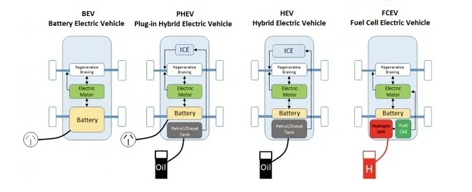
There are 4 types of electric cars, with the following outline:-

• Battery Electric Vehicle (BEV)
• Hybrid Electric Vehicle (HEV)
• Plug-in Hybrid Electric Vehicle (PHEV)
• Fuel Cell Electric Vehicle (FCEV)

In brief, the system architecture of the four types of electric cars can be seen in the following figure:-

Battery Electric Vehicle (BEV):-

A Battery Electric Vehicle (BEV), also called All-Electric Vehicle (AEV), runs entirely on a battery and electric drive train. These types of electric cars do not have an ICE. Electricity is stored in a large battery pack that is charged by plugging into the electricity grid. The battery pack, in turn, provides power to one or more electric motors to run the electric car.

Architecture and main components of BEV are:-

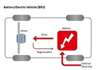
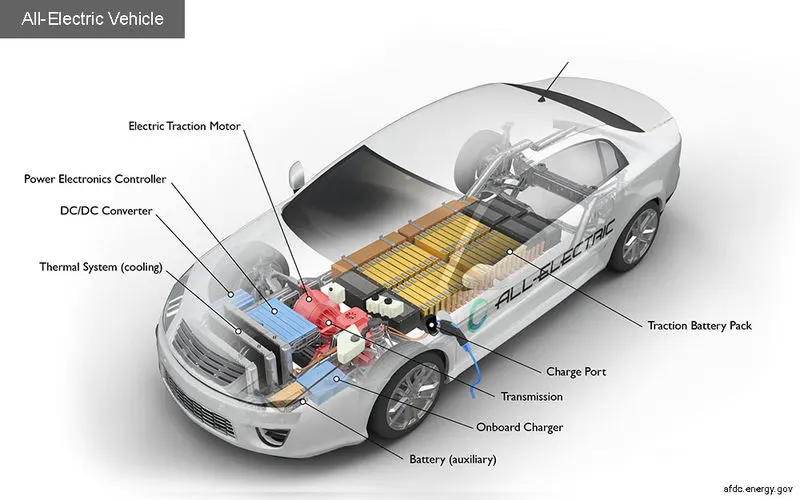
Components of BEV are:-

• Electric Motor
• Inverter
• Battery
• Control Module
• Drive train

Working Principles of BEV are:-

• Power is converted from the DC battery to AC for the electric motor.
• The accelerator pedal sends a signal to the controller which adjusts the vehicle’s speed by changing the frequency of the AC power from the inverter to the motor.
• The motor connects and turns the wheels through a cog.
• When the brakes are pressed or the electric car is decelerating, the motor becomes an alternator and produces power, which is sent back to the battery.

Examples of BEV:-

• Volkswagen e-Golf, Tesla Model 3, BMW i3, Chevy Bolt, Chevy Spark, Nissan LEAF, Ford Focus Electric, Hyundai Ioniq, Karma Revera, Kia Soul, Mitsubishi i-MiEV, Tesla X, Toyota Rav4.

Hybrid Electric Vehicle (HEV):-

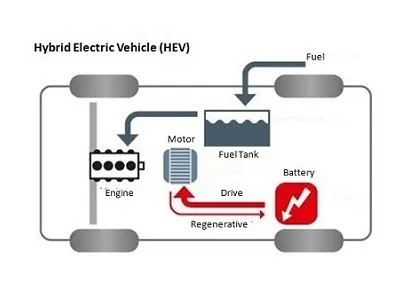
• This type of hybrid car is often called a standard hybrid or parallel hybrid. HEV has both an ICE and an electric motor. In these types of electric cars, the internal combustion engine gets energy from fuel (gasoline and others type of fuels), while the motor gets electricity from batteries. The gasoline engine and electric motor simultaneously rotate the transmission, which drives the wheels.
• The difference between HEV compared to BEV and PHEV is where the batteries in HEV can only charge by the ICE, the motion of the wheels, or a combination of both. There is no charging port so that the battery cannot be recharged from outside of the system, for example from the electricity grid.

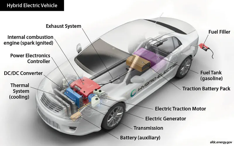
Architecture and main components of HEV are:-

Components of HEV are:-

• Engine
• Electric Motor
• Battery Pack with controller & inverter
• Fuel Tank
• Control Module

Working Principles of HEV:-

• Has a fuel tank that supplies gas to the engine like a regular car.
• It also has a set of batteries that run an electric motor.
• Both the engine and electric motor can turn the transmission at the same time.

Examples of HEV:-

• Honda Civic Hybrid, Toyota Prius Hybrid, Honda Civic Hybrid, Toyota Camry Hybrid.

Plug-in Hybrid Electric Vehicle (PHEV):-

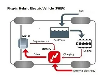
PHEV is a type of hybrid vehicle that is both an ICE and a motor, often called a series hybrid. This type of electric car offers a choice of fuels. This type of electric car is powered by a conventional fuel (such as gasoline) or an alternative fuel (such as bio-diesel) and by a rechargeable battery pack. The battery can be charged up with electricity by plugging into an electrical outlet or electric vehicle charging station (EVCS).

PHEV typically can run in at least two modes:

• All-electric Mode, in which the motor and battery provide all the car’s energy
• Hybrid Mode, in which both electricity and gasoline are employed.

Some PHEVs can travel more than 70 miles on electricity alone.

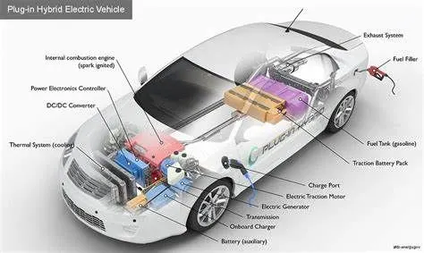
Architecture and main components of PHEV are:-

Components of PHEV are:-

• Electric Motor
• Engine
• Inverter
• Battery
• Fuel Tank
• Control Module
• Battery Charger (If onboard model)

Working Principles of PHEV are:-

• PHEVs typically start-up in all-electric mode and operate on electricity until their battery pack is depleted. Some models shift to hybrid mode when they reach highway cruising speed, generally above 60 or 70 miles per hour. Once the battery is empty, the engine takes over and the vehicle operates as a conventional, non-plug-in hybrid.
• In addition to plugging into an outside electric power source, PHEV batteries can be charged by an internal combustion engine or regenerative braking. During braking, the electric motor acts as a generator, using the energy to charge the battery. The electric motor supplements the engine’s power; as a result, smaller engines can be used, increasing the car’s fuel efficiency without compromising performance.

Examples of PHEV:-

• Porsche Cayenne S E-Hybrid, Chevy Volt, Chrysler Pacifica, Ford C-Max Energi, Ford Fusion Energi, Mercedes C350e, Mercedes S550e, Mercedes GLE550e, Mini Cooper SE Countryman, Audi A3 E-Tron, BMW 330e, BMW i8, BMW X5 xdrive40e, Fiat 500e, Hyundai Sonata, Kia Optima, Porsche Panamera S E-hybrid, Volvo XC90 T8.

Fuel Cell Electric Vehicle (FCEV):-

• Fuel Cell Electric Vehicles (FCEVs), also known as fuel cell vehicles (FCVs) or Zero Emission Vehicle, are types of electric cars that employ ‘fuel cell technology to generate the electricity required to run the vehicle. In this type of vehicle, the chemical energy of the fuel is converted directly into electric energy.

Architecture and main components of FCEV are:-

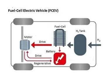
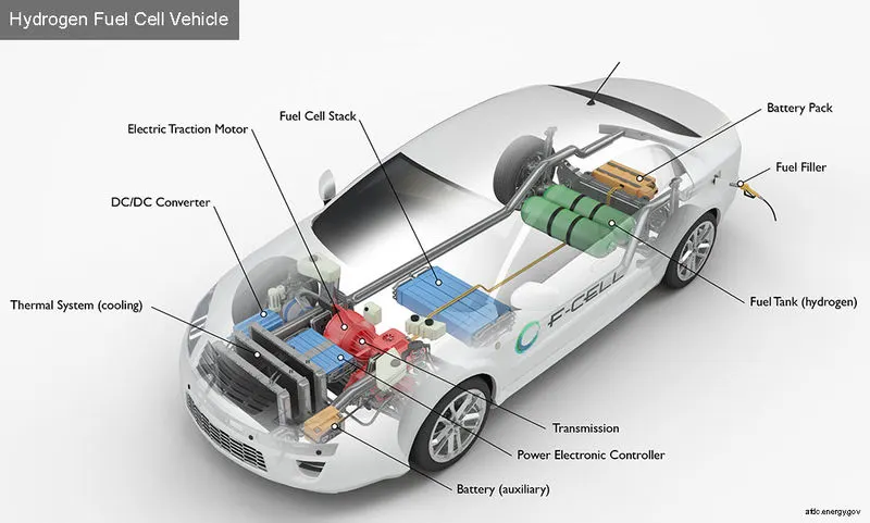
Components of FCEV are:-

• Electric Motor
• Fuel-cell stack
• Hydrogen Storage Tank
• Battery with controller and converter

Working Principles of FCEV:-

• The working principle of a ‘fuel cell’ electric car is different compared to that of a ‘plug-in’ electric car. This type of electric car is because the FCEV generates the electricity required to run this vehicle on the vehicle itself.

Examples of FCEV are:-

• Toyota Mirai, Hyundai Tucson FCEV, Riversimple Rasa, Honda Clarity Fuel Cell, Hyundai Nexo.

BLOCK DIAGRAM:-

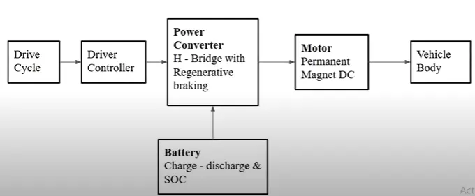
Important Simulink Block used in Electric Vehicle Design are:

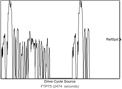
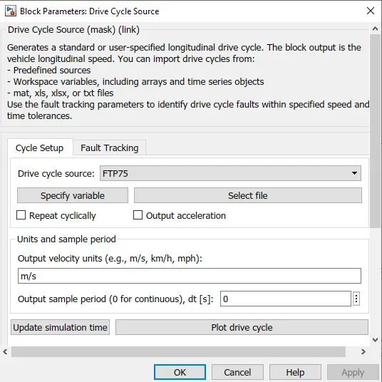
1). Drive Cycle Source:- The Drive Cycle Source block generates a standard or user-specified longitudinal drive cycle. The block output is the specified vehicle longitudinal speed, which you can use to:

• Predict the engine torque and fuel consumption that a vehicle requires to achieve desired speed and acceleration for a given gear shift reference.
• Produce realistic velocity and shift references for closed-loop acceleration and braking commands for vehicle control and plant models.
• Study, tune, and optimize vehicle control, system performance, and system robustness over multiple drive cycles.
• Identify the faults within tolerances specified by standardized tests, including:

1). EPA dynamometer driving schedules

2). Worldwide Harmonized Light Vehicle Test Procedure (WLTP) laboratory tests

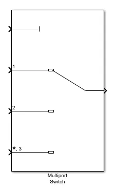
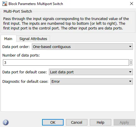
2). Multiport Switch:- The Multiport Switch block determines which of several inputs to the block passes to the output. The block bases this decision on the value of the first input. The first input is the control input and the remaining inputs are the data inputs. The value of the control input determines which data input passes to the output.

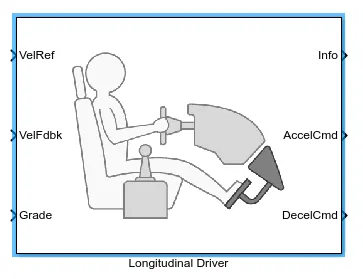
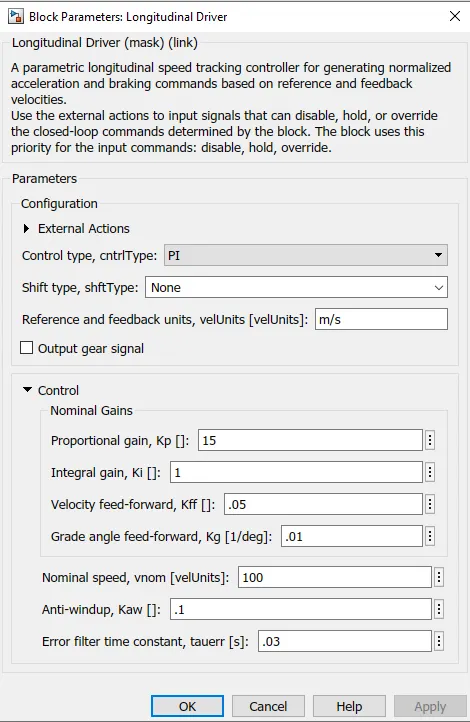
3). Longitudinal Driver:- The Longitudinal Driver block implements a longitudinal speed-tracking controller. Based on reference and feedback velocities, the block generates normalized acceleration and braking commands that can vary from 0 through 1. You can use the block to model the dynamic response of a driver or to generate the commands necessary to track a longitudinal drive cycle.

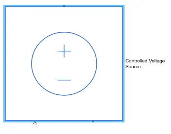
4). Controlled Source:- The Controlled Voltage Source block represents an ideal voltage source that is powerful enough to maintain the specified voltage at its output regardless of the current flowing through the source. The output voltage is V = Vs, where Vs is the numerical value presented at the physical signal port.

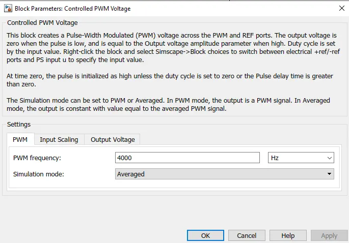
5). Controlled PWM Voltage:- The Controlled PWM Voltage block represents a pulse-width modulated (PWM) voltage source. The block has two modeling variants, accessible by right-clicking the block in your block diagram and then selecting the appropriate option from the context menu, under Simscape > Block choices:

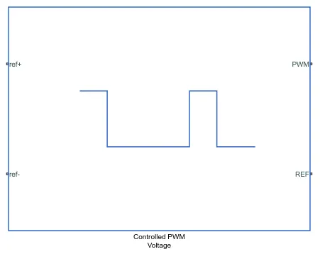
• Electrical input ports — The block calculates the duty cycle based on the reference voltage across its ref+ and ref- ports. This modeling variant is the default.
• PS input — Specify the duty cycle value directly by using an input physical signal port.

For the Electrical input ports variant of the block, the demanded duty cycle is

100∗Vref−VminVmax−Vmin percent

where:

• V_ref is the reference voltage across the ref+ and ref- ports.
• V_min is the minimum reference voltage.
• V_max is the maximum reference voltage.

The value of the Output voltage amplitude parameter determines the amplitude of the output voltage.

At time zero, the pulse is initialized as high, unless the Pulse delay time parameter is greater than zero, or the demanded duty cycle is zero.

You can use parameters Pulse delay time and Pulse width offset to add a small turn-on delay and a small turn-off advance. This can be useful when fine-tuning switching times so as to minimize switching losses.

In PWM mode, the block has two options for the type of switching event when moving between output high and output low states:

• Asynchronous – Best for variable-step solvers — Asynchronous events are better suited to variable step solvers because they require fewer simulation steps for the same level of accuracy. In asynchronous mode, the PWM switching events generate zero crossings, and therefore switching times are always determined accurately, regardless of the simulation maximum step size.
• Discrete-time – Best for fixed-step solvers — Discrete-time events are better suited to fixed-step operation because then the switching events are always synchronized with the simulation step. Using an asynchronous implementation with fixed-step solvers may sometimes result in events being up to one simulation step late.

If you use a fixed-step or local solver and the discrete-time switching event type, the following restrictions apply to the Sample time parameter value:

• The sample time must be a multiple of the simulation step size.
• The sample time must be small compared to the PWM period, to ensure sufficient resolution.

Assumptions and Limitations: -

The model is based on the following assumptions:

• The REF output of this block is floating, it is not tied to the Electrical Reference. One consequence of this is that if you connect the PWM and REF electrical ports directly to the PWM and REF electrical ports of an H-bridge or a gate driver, you must attach an Electrical Reference block to the REF connection line.
• Do not connect the Controlled PWM block directly to a semiconductor gate, because this omits the gate driver output impedance that determines switching dynamics. Use a Gate Driver or a Half-Bridge Driver block to set the gate source or the gate-emitter voltage.
• Do not use the Controlled PWM block to drive a motor block directly. A PWM motor driver goes open circuit in between pulses. Use the H-Bridge block to drive a motor block.
• When driving a motor via the H-Bridge block, set the Simulation mode parameter to Averaged to speed up simulations. You must also set the Simulation mode parameter of the H-Bridge block to Averaged mode. This applies the average of the demanded PWM voltage to the motor. The Averaged mode assumes that the impedance of the motor inductive term is small at the PWM frequency. To verify this assumption, run the simulation using the PWM mode and compare the results to those obtained from using the Averaged mode.
• If you are linearizing your model, set the Simulation mode parameter to Averaged and ensure that you have specified the operating point of the block correctly. You can only linearize the block for inputs corresponding to a duty cycle greater than zero and less than 100 percent.
• When you use this block in PWM mode with the Use local solver option selected in the Solver Configuration block, set the Switching event type parameter to Discrete-time – Best for fixed-step solvers. Using the Asynchronous – Best for variable-step solvers option in this situation may produce inaccuracies because simulation with the local solver implies fixed step, and the PWM events will not always coincide precisely with the simulation steps. This results in PWM events sometimes occurring one simulation step late.

6). H-Bridge:- The H-Bridge block represents an H-bridge motor driver. The block has the following two Simulation mode options:

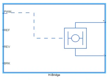
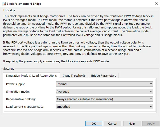
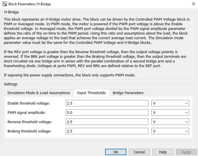
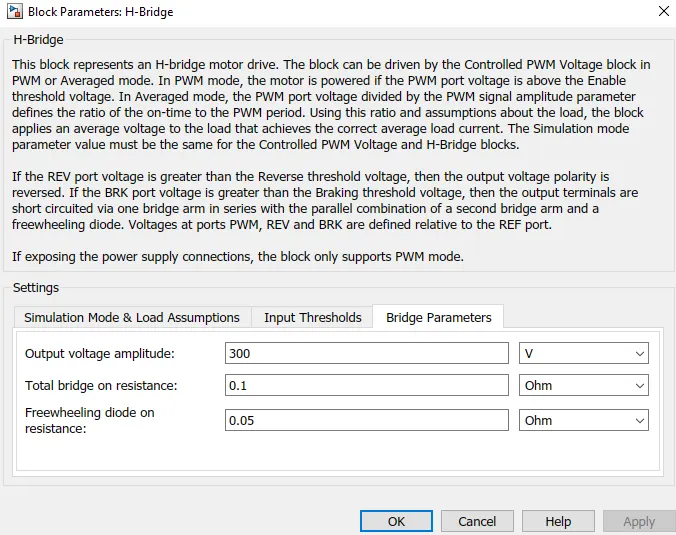
• PWM — The H-Bridge block output is a controlled voltage that depends on the input signal at the PWM port. If the input signal has a value greater than the Enable threshold voltage parameter value, the H-Bridge block output is on and has a value equal to the value of the Output voltage amplitude parameter. If it has a value less than the Enable threshold voltage parameter value, the block maintains the load circuit using one of the following three Freewheeling mode options:
• Via one semiconductor switch and one freewheeling diode
• Via two freewheeling diodes
• Via two semiconductor switches and one freewheeling diode

The first and third options are sometimes referred to as synchronous operations.

The signal at the REV port determines the polarity of the output. If the value of the signal at the REV port is less than the value of the Reverse threshold voltage parameter, the output has positive polarity; otherwise, it has negative polarity.

• Averaged — This mode has two Load current characteristics options:
• Smoothed
• Unsmoothed or discontinuous

The Smoothed option assumes that the current is practically continuous due to load inductance. In this case, the H-Bridge block output is:

`(V_oV_(PWM))/A_(PWM)-I_(OUT)R_(ON)`

where:

• V_O is the value of the Output voltage amplitude parameter.
• V_PWM is the value of the voltage at the PWM port.
• A_PWM is the value of the PWM signal amplitude parameter.
• I_OUT is the value of the output current.
• R_ON is the Bridge on the resistance parameter.

The current will be smooth if the PWM frequency is large enough. Synchronous operation where freewheeling is via a bridge arm back to the supply also helps smooth the current. For cases where the current is not smooth, or possibly discontinuous (that is, it goes to zero between PWM cycles), use the Unsmoothed or discontinuous option. For this option, you must also provide values for the Total load series resistance, Total load series inductance, and PWM frequency. During simulation, the block uses these values to calculate a more accurate value for H-bridge output voltage that achieves the same average current as would be present if simulating in PWM mode.

Set the Simulation mode parameter to Averaged to speed up simulations when driving the H-Bridge block with a Controlled PWM Voltage block. You must also set the Simulation mode parameter of the Controlled PWM Voltage block to Averaged mode. This applies the average of the demanded PWM voltage to the motor. The accuracy of the Averaged mode simulation results relies on the validity of your assumption about the load current. If you specify that the current is Unsmoothed or discontinuous, then the accuracy also depends on the values you provide for load resistance and inductance being representative. This mode also makes some simplifying assumptions about the underlying equations for the case when the current is discontinuous. For typical motor and bridge parameters, accuracy should be within a few percent. To verify Averaged mode accuracy, run the simulation using the PWM mode and compare the results to those obtained from using the Averaged mode.

Braking mode is invoked when the voltage presented at the BRK port is larger than the Braking threshold voltage. Regardless of whether in PWM or Averaged mode, when in braking mode the H-bridge is modeled by a series combination of two resistances R1 and R2 where:

• R1 is the resistance of a single bridge arm, that is, half the value of the Total bridge on the resistance parameter.
• R2 is the resistance of a single bridge arm in parallel with a diode resistance, that is, R1 · Rd / (R1 + Rd), where Rd is the diode resistance.

Assumptions and Limitations: -

• If you are linearizing your model, set the Simulation mode parameter to Averaged and ensure that you have specified the operating point correctly. You can only linearize the H-Bridge block for duty cycles that are greater than zero and less than the PWM signal amplitude. If you need to linearize around zero duty cycle, and if your controller always uses regenerative braking mode, set the Regenerative braking parameter to Always enabled (suitable for linearization).
• In Averagedmode, and with the Unsmoothed or discontinuous choice for Load current characteristics, you must provide representative values for load inductance and resistance. If driving a DC Motor, then the resistance is the armature resistance, and the inductance is the sum of the armature inductance plus series smoothing inductor (if present). For a Universal Motor, the total resistance is the sum of the armature and field windings, and total inductance is the sum of armature and field inductances plus any series smoothing inductance. For a Shunt Motor, MathWorks recommends that you draw a Thevenin equivalent circuit to determine appropriate values.
• No forward voltage is modeled for the freewheeling diodes. They are approximated as ideal resistances when forward biased, with resistance equal to the Freewheeling diode on the resistance parameter value.
• If the supply rail connections are exposed, only the PWM simulation mode is supported.

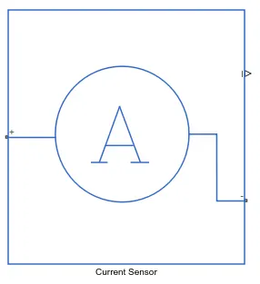
7). Current Sensor:- The Current Sensor block represents an ideal current sensor, that is, a device that converts current measured in any electrical branch into a physical signal proportional to the current. Connections + and – are electrical conserving ports through which the sensor is inserted into the circuit. The connection I am a physical signal port that outputs the measurement result.

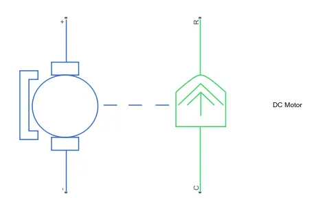
8). DC Motor:- The DC Motor block represents the electrical and torque characteristics of a DC motor using the following equivalent circuit model:

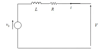
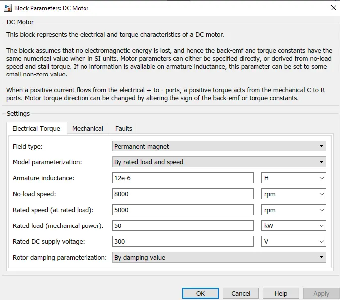
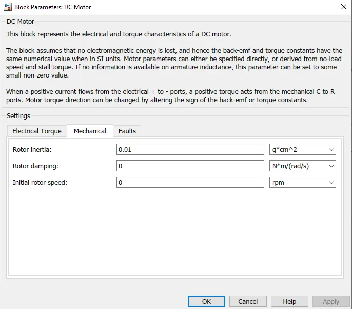
You specify the equivalent circuit parameters for this model when you set the Model parameterization parameter to by equivalent circuit parameters. The resistor R corresponds to the resistance you specify in the Armature resistance parameter. The inductor L corresponds to the inductance you specify in the Armature inductance parameter.

You can specify how to generate the magnetic field of the DC motor by setting the Field type parameter to the desired option. The permanent magnets in the motor induce the following back emf `v_b` in the armature:

`v_b=k_vω`

where `k_v` is the Back-emf constant and ω is the angular velocity. The motor produces the following torque, which is proportional to the motor current i:

`T_E=k_ti`

where `k_t` is the Torque constant. The DC Motor block assumes that there are no electromagnetic losses. This means that mechanical power is equal to the electrical power dissipated by the back emf in the armature. Equating these two terms gives:

`T_Eω=v_bi`

`k_tiω=k_vωi`

`k_v=k_t`

As a result, you specify either `k_v`or `k_t` in the block parameters.

If the magnetic field is generated from the current flowing through the windings, the Back-emf constant depends on the field current `I_f`:

`k_v=L_(af)I_f`

where `L_(af)` is the Field-armature mutual inductance.

The torque-speed characteristic for the DC Motor block is related to the parameters in the preceding figure. When you set the Model parameterization parameter to by stall torque & no-load speed or by rated power, rated speed & no-load speed, the block solves for the equivalent circuit parameters as follows:

1. For the steady-state torque-speed relationship, L has no effect.
2. Sum the voltages around the loop and rearrange for i:

`I =(V−v_b)/R=(V−k_vω)/R`

3. Substitute this value of i into the equation for torque:

`T_E=k_t/R(V−k_vω)`

When you set the Model parameterization parameter to by stall torque & no-load speed, the block uses the preceding equation to determine values for R and _{k_t} (and equivalently `k_v`).

When you set the Model parameterization parameter to by rated power, rated speed & no-load speed, the block uses the rated speed and power to calculate the rated torque. The block uses the rated torque and no-load speed values in the preceding equation to determine values for R and `k_t`.

The block models motor inertia J and damping `lamda` for all values of the Model parameterization parameter. The resulting torque across the block is:

`T=k_t/R(V−kvω) −Jdotω−lamdaω`

It is not always possible to measure rotor damping, and rotor damping is not always provided on a manufacturer datasheet. An alternative is to use the no-load current to infer a value for rotor damping.

For no-load, the electrically-generated mechanical torque must equal the rotor damping torque:

`k_ti_(noload)=λω_(noload)`

where `i_(noload)` is the no-load current. If you select by the no-load current for the Rotor damping parameterization parameter, then this equation is used in addition to the torque-speed equation to determine values for λ and the other equation coefficients.

The value for rotor damping, whether specified directly or in terms of no-load current, is taken into account when determining equivalent circuit parameters for Model parameterization options By stall torque and no-load speed and By rated power, rated speed, and no-load speed.

When a positive current flows from the electrical + to - ports, a positive torque acts from the mechanical C to R ports.

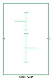
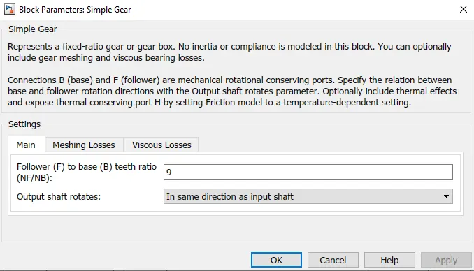
9). Simple Gear:- The Simple Gear block represents a gearbox that constrains the connected driveline axes of the base gear, B, and the follower gear, F, to corotate with a fixed ratio that you specify. You choose whether the follower axis rotates in the same or opposite direction as the base axis. If they rotate in the same direction, the angular velocity of the follower, ω_F, and the angular velocity of the base, ω_B, have the same sign. If they rotate in opposite directions, ω_F and ω_B have opposite signs.

Ideal Gear Constraint and Gear Ratio

The kinematic constraint that the Simple Gear block imposes on the two connected axes is

`r_Fω_F=r_Bω_B`

where:

• `r_F`is the radius of the follower gear.
• `omega_F`is the angular velocity of the follower gear.
• `r_B`is the radius of the base gear.
• `omega_B`is the angular velocity of the base gear.

The follower-base gear ratio is

`g_(FB)=r_F/r_B=N_F/N_B`

where:

• `N_B`is the number of teeth in the base gear.
• `N_(BF)` is the number of teeth in the follower gear.

Reducing the two degrees of freedom to one independent degree of freedom yields the torque transfer equation

`g_(FB)tau_B+tau_F−tau_(loss)=0`

where:

• `tau_B`is the input torque.
• `tau_F`is the output torque.
• `tau_(loss)`is the torque loss due to friction.

For the ideal case, `tau_(loss)`=0.

Nonideal Gear Constraint and Losses

In the nonideal case, `tau_(loss)≠0`. For general considerations on nonideal gear modeling.

In a nonideal gear pair (B, F), the angular velocity, gear radii, and gear teeth constraints are unchanged. But the transferred torque and power are reduced by:

• Coulomb friction between teeth surfaces on gears Band F, characterized by efficiency, `eta`
• Viscous coupling of driveshafts with bearings, parametrized by viscous friction coefficients, `mu`

Constant Efficiency

In the constant efficiency case, `eta` is constant, independent of load or power transferred.

Load-Dependent Efficiency

In the load-dependent efficiency case, `eta` depends on the load or power transferred across the gears. For either power flow,

`tau_(Cou l)=g_(FB)tau_(idl e)+ktau_F`

where:

• `tau_(Cou l)`is the Coulomb friction dependent torque.
• `k`is a proportionality constant.
• `tau_(idl e)`is the net torque acting on the input shaft in idle mode.

Efficiency, `eta`, is related to `tau_(Cou l)` in the standard, preceding form but becomes dependent on load:

`eta=tau_F/(g_(FB)tau_(idl e)+(k+1)tau_F`

10). Tire (Magic Formula):- The Tire (Magic Formula) block models a tire with longitudinal behavior given by the Magic Formula [1], an empirical equation based on four fitting coefficients. The block can model tire dynamics under constant or variable pavement conditions.

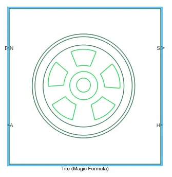
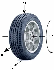
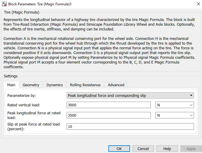
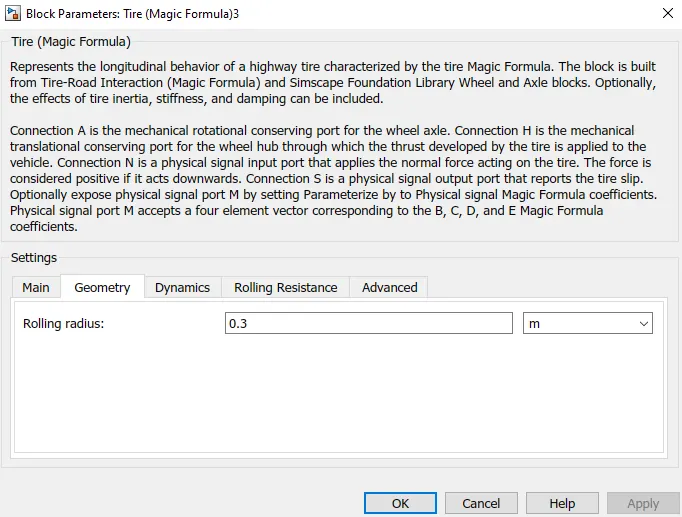
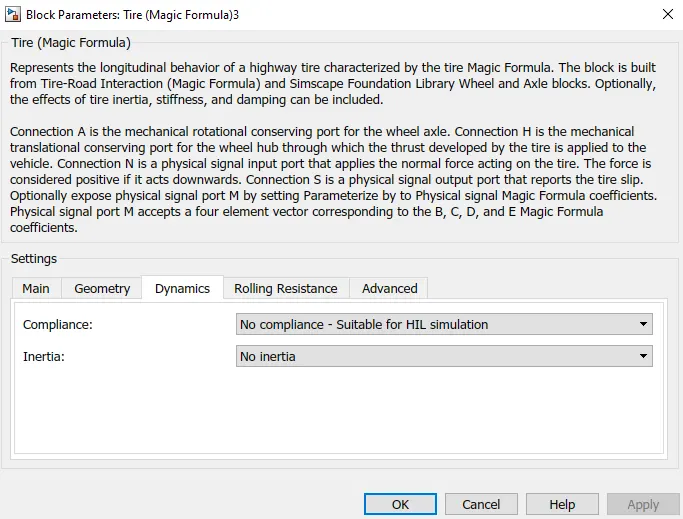
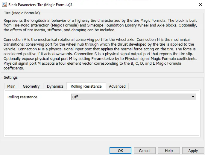
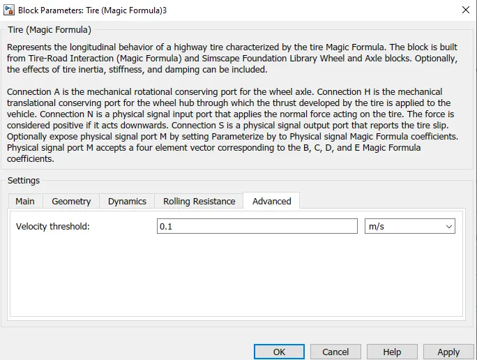
The longitudinal direction of the tire is the same as its direction of motion as it rolls on the pavement. This block is a structural component based on the Tire-ROad Interaction (Magic Formula) block.

To increase the fidelity of the tire model, you can specify properties such as tire compliance, inertia, and rolling resistance. However, these properties increase the complexity of the tire model and can slow down the simulation. Consider ignoring tire compliance and inertia if simulating the model in real-time or if preparing the model for hardware-in-the-loop (HIL) simulation.

Tire Model

The Tire (Magic Formula) block models the tire as a rigid wheel-tire combination in contact with the road and subject to slip. When torque is applied to the wheel axle, the tire pushes on the ground (while subject to contact friction) and transfers the resulting reaction as a force back on the wheel. This action pushes the wheel forward or backward. If you include the optional tire compliance, the tire also flexibly deforms under load.

The figure shows the forces acting on the tire. The table defines the tire model variables.

Assumptions and Limitations

• The Tire (Magic Formula) block assumes longitudinal motion only and includes no camber, turning, or lateral motion.
• Tire compliance implies a time lag in the tire response to the forces on it. Time lag simulation increases model fidelity but reduces simulation performance.

11). Vehicle Body:- The Vehicle Body block represents a two-axle vehicle body in longitudinal motion. The vehicle can have the same or a different number of wheels on each axle. For example, two wheels on the front axle and one wheel on the rear axle. The vehicle wheels are assumed identical in size. The vehicle can also have a center of gravity (CG) that is at or below the plane of travel.

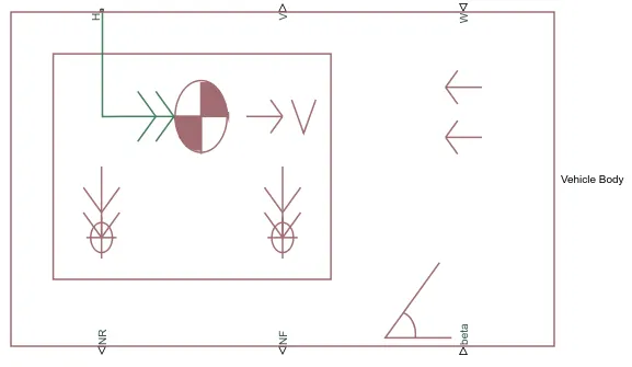
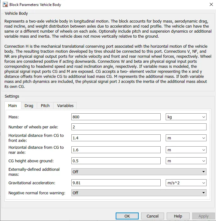
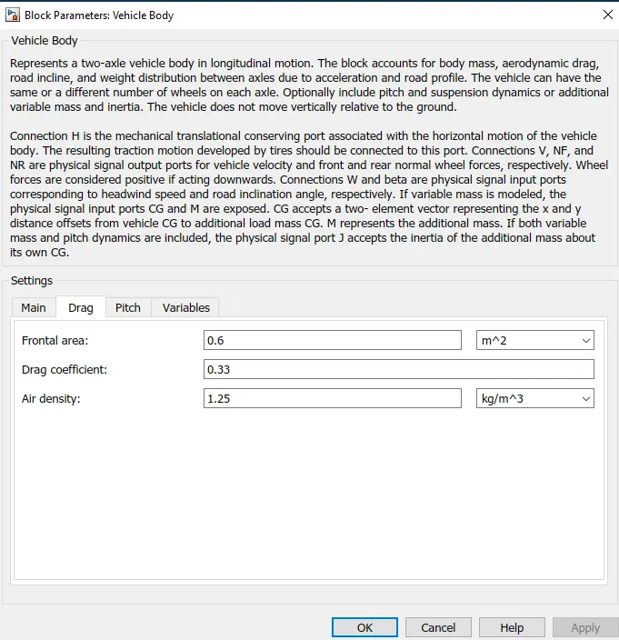
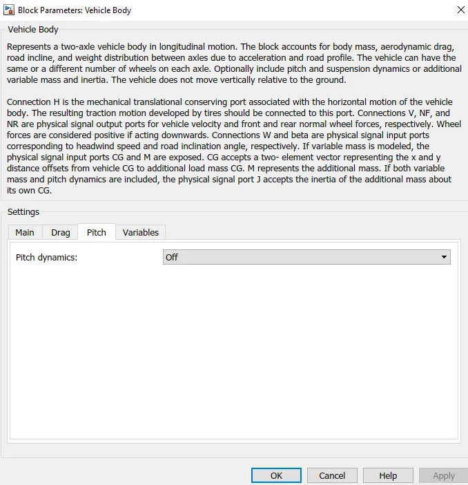
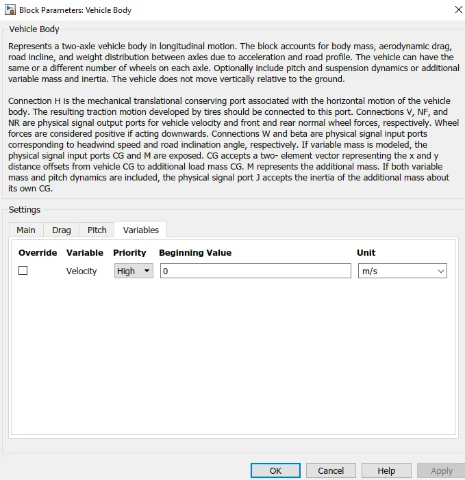
The block accounts for body mass, aerodynamic drag, road incline, and weight distribution between axles due to acceleration and road profile. Optionally include pitch and suspension dynamics. The vehicle does not move vertically relative to the ground.

The block has an option to include an externally-defined mass and externally-defined inertia. The mass, inertia, and center of gravity of the vehicle body can vary over the course of simulation in response to system changes.

Model

The vehicle axles are parallel and form a plane. The longitudinal, x, direction lies in this plane and perpendicular to the axles. If the vehicle is traveling on an inclined slope, β, the normal, z, the direction is not parallel to gravity but is always perpendicular to the axle-longitudinal plane.

This figure and table define the vehicle motion model variables.

Vehicle Dynamics and Motion:-

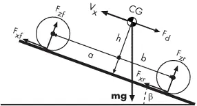
This block contains 6 ports that can be used in various aspects:

• H-H stand for hub it is used to connect the hub of wheels to the main body of the vehicle.
• The V-Physical signal output port of velocity is used as the velocity output of the vehical.
• W-Physical input port used to wind velocity acts against the vehicle.
• NR- Physical signal output port used to connect the rare wheels.
• NF- Physical signal output port used to connect the front wheels.
• Beta- Physical signal input port that allows the vehicle to undergo an inclination of hill-climbing force.

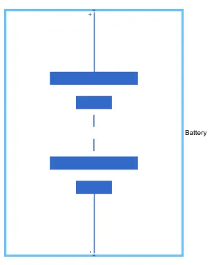
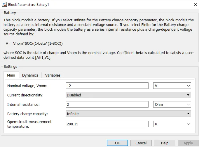
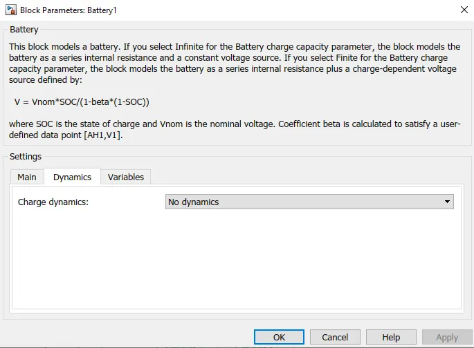
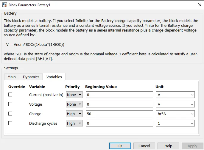
12). Battery:- The Battery block represents a simple battery model. The block has four modeling variants, accessible by right-clicking the block in your block diagram and then selecting the appropriate option from the context menu, under Simscape > Block choices:

• Un instrumented | No thermal port— A basic model that does not output battery charge level or simulates thermal effects. This modeling variant is the default.
• Un instrumented | Show thermal port— Model with exposed thermal port. This model does not measure the internal charge level of the battery.
• Instrumented | No thermal port— Model with an exposed charge output port. This model does not simulate thermal effects.
• Instrumented | Show thermal port— Model that lets you measure the internal charge level of the battery and simulate thermal effects. Both the thermal port and the charge output port are exposed.

The instrumented variants have an extra physical signal port that outputs the internal state of charge. Use this functionality to change load behavior as a function of the state of charge, without the complexity of building a charge state estimator.

The thermal port variants expose a thermal port, which represents the battery thermal mass. When you select this option, provide additional parameters to define battery behavior at a second temperature. For more information.

The battery equivalent circuit is made up of the fundamental battery model, the self-discharge resistance `R_(SD)`, the charge dynamics model, and the series resistance `R_0.`

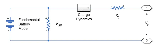
Battery Model:-

If you select Infinite for the Battery charge capacity parameter, the block models the battery as a series resistor and a constant voltage source. If you select Finite for the Battery charge capacity parameter, the block models the battery as a series resistor and a charge-dependent voltage source. In the finite case, the voltage is a function of charge and has the following relationship:

`V=V_0((SOC)/(1-beta(1-SOC)))`

where:

• SOC (state-of-charge) is the ratio of current charge to-rated battery capacity.
• `V_0`is the voltage when the battery is fully charged at no load, as defined by the Nominal voltage,` V_(nom)`
• `beta` is a constant that is calculated so that the battery voltage is V1 when the charge is AH1. Specify the voltage V1 and ampere-hour rating AH1 using block parameters. AH1 is the charge when the no-load (open-circuit) voltage is V1, and V1 is less than the nominal voltage.

The equation defines an approximate relationship between voltage and the remaining charge. This approximation replicates the increasing rate of voltage drop at low charge values and ensures that the battery voltage becomes zero when the charge level is zero. The advantage of this model is that it requires few parameters, which are readily available on most datasheets.

By using MATLAB SIMULINK system block for Electric Vehicle Design are:-

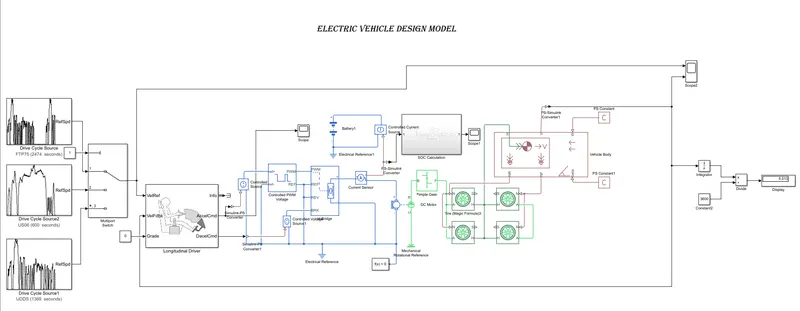
STATE OF CHARGE (SOC):-

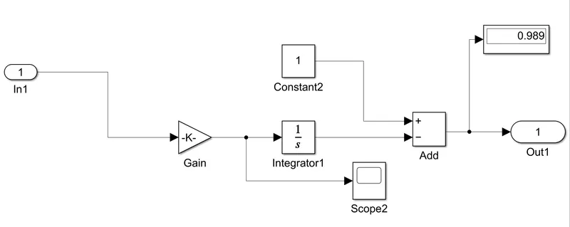
To measure the state of charge of the battery, the integrator block is used to handle data transfer and integrate the value of the current signal with respect to time then gain block is used to multiply divide the signal coming from the integrating block. This block will divide a current signal with the ampere rating battery which is 160(ah)*3600 (sec). Assuming the battery is always fully charged I have added a constant block with a value of 1 representing 100%.

RESULTS:-

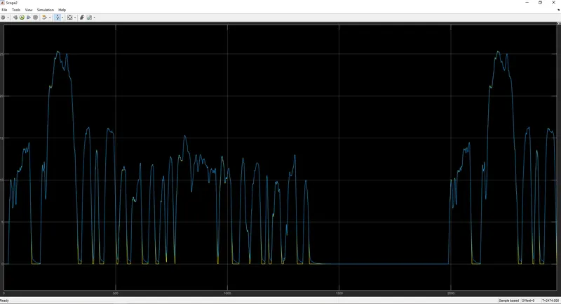
The output of the drive cycle and velocity graph can be seen and observed that the velocity depends on the drive cycle input.

SOC output graph snapshot given below:-

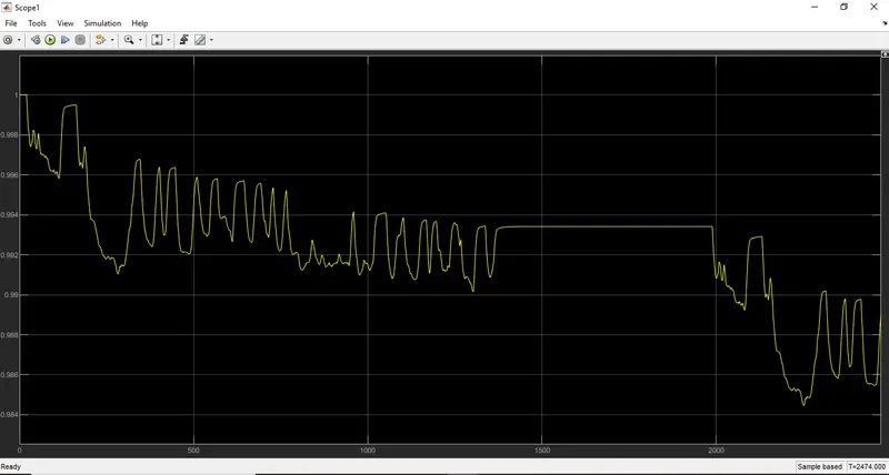
In this graph state of charge of the battery decreases with time. In the SOC graph the speed spikes show regenerative braking is considered.

CONCLUSION:-

The EV model has been created successfully with Simulink and the model simulated with Drive Cycle source FTP75 (2474 seconds) the simulation has produced the results of vehicle with respect to acceleration and current flowing state of charge as well as the distance traveled in simulation time.