Parametric study on Gate valve.

Aim - To perform a parametric study on the gate valve simulation by setting the opening from 10 % to 80%.
• Obtain the mass flow rates at the outlet for each design point.
• Calculate the flow coefficient and flow factor for each opening and plot the graph.
• Discuss the results of the mass flow rate and flow coefficient.

Objective –
• The main objective of this challenge is to set up steady-state simulations of water flow through a gate valve.
• To perform simulation for various gate valve openings from 10% to 80%
• Perform a parametric study
• Compare Mass flow rate, Flow coefficient and flow factor.

Introduction –
This project involves simulating a steady state water flow inside a gate valve for a range of openings from 10% to 80%. Only one instance is simulated, and the remainder simulation is carried out using a parametric analysis. A parameter for opening distance is set. In order to investigate the internal flow of the water, velocity and pressure vector distributions are displayed. In order to comprehend how the flow behaves for the various openings of the gate valve, the mass flow rate, flow coefficient, and flow factor are computed and compared.

Theory –
Gate Valve:
A gate valve is a particular kind of valve that controls the flow of fluid in pipework by moving a gate- or wedge-type disc perpendicular to the flow. The most typical type of valve found in any process plant is a gate valve. It is a linear motion valve that controls when fluid flow begins or stops. These valves are either fully open or totally closed when in use. A gate valve's disc is entirely cut off from the flow when it is fully opened. There is therefore almost minimal flow resistance. As a result, the pressure drop that occurs when fluid passes through a gate valve is minimal.
When the valve is fully closed, the disc and seats must make 360° of surface contact in order to establish good sealing. As precise control is not achievable, gate valves should not be utilised to regulate or throttle flow. The disc and seating surfaces may erode due to the partially open valve's high flow velocity, which can also generate vibration and noise.

Types of Gate Valves:
1. Types of Disk
a. Solid taper wedge
b. Flexible wedge
c. Split wedge or Parallel disks Valve
2. Types of Body Bonnet Joint
a. Screwed Bonnet
b. Bolted-Bonnet
c. Welded-Bonnet
d. Pressure-Seal Bonnet
3. Types of Stem movement
a. Rising Stem or OS & Y Type (Outside Stem and Screw Type)
b. Non-rising Stem type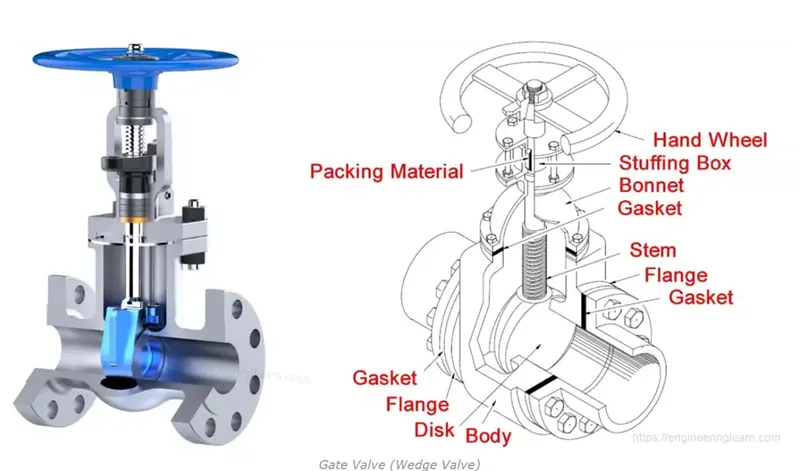

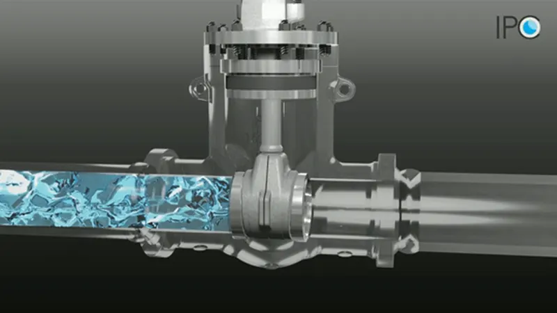
Similar to other valves, a gate valve also functions. Turning the handwheel raises or lowers the gate on the stem via the threads, opening the valve. For a gate valve to fully open or close, it takes more than one 360° rotation. The inlet and exit are opened when the gate is raised, providing the media with an unhindered path of travel. The gate closes and obstructs the flow of media when it is lowered.

Gate Valve Applications:
• Almost all fluid services, including air, fuel gas, feedwater, steam, lubricant oil, hydrocarbon, and nearly any other services, employ gate valves.
• Slurry and powder products also use specialised gate valves, such as knife gate valves.
Advantages of Gate Valve:
• Gate valve offers effective cut-off
• There is extremely little pressure loss during operation.
• Most gate valves can be utilised in a bi-directional fashion.
• They require minimal maintenance and are appropriate for applications involving high pressure and temperature.

Disadvantages of Gate Valve:
• The flow cannot be managed using it.
• A gate valve operates slowly. It is advantageous that opening and closing take time since it lessens the possibility of pounding.
• When only partially open, it vibrates and makes noise.
• Due of the restricted access, repairs like lapping and grinding of seats are more challenging.

Parametric Study:
Effectively supporting product concept designs is a parametric study that modifies design factors in the product design model to investigate design alternatives. As long as the mapping between the simulation and CAD models has been established, a parametric analysis is straightforward and simple to carry out. Fast simulation model development for performance analyses is supported by the mapping. Additionally, it supports the finite difference approach for DSA. Concept design allows for the parametric research because there are typically few design factors to perturb.
One of the main problems facing engineers, especially those who use FE software, is parameter optimisation. Sometimes it's necessary to look into design factors that are influencing results in addition to mesh characteristics. Changing the model every time and running the analysis again takes a lot of time. Fortunately, Ansys enables users to optimise their models without having to reinvent them or run them repeatedly. You can expose several parameters to the user via parameter sets. Additionally, to return various information based on the user-specified parameters.

Flow Coefficient:
A device's relative ability to permit fluid flow is measured by the flow coefficient. It explains the connection between the corresponding flow rate and the pressure drop via an orifice valve or other component. The flow coefficient, often known as the flow capacity rating CV, can be stated mathematically as,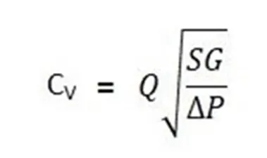

Where ,
Q is the rate of flow (gallons per minute)
SG is the specific gravity of fluid (for water =1)
ΔP is the pressure drop across the valve expressed in psi.
10 Pa = 0.00145038 psi
In more concrete terms, the flow coefficient Cv is the amount of water (in US gallons) at 60 °F that will pass through a valve once there is a 1 psi pressure decrease across the valve each minute. The industry accepts the use of the flow coefficient as a common method for comparing valve capacity and sizing valves for particular applications.

Flow Factor:
The valve capacity is simply stated by the constant known as the Kv-factor for a specific valve. The valve manufacturer runs experiments to ascertain the Kv-factor. The Kv factor determines the amount of water that will flow through the valve in m3 per hour at a pressure drop of 1 Bar.
Metric measurements are used to determine the metric equivalent flow factor (Kv). Metric units are used to calculate the metric equivalent of the Kv factor, which is widely used in Europe and the Asia.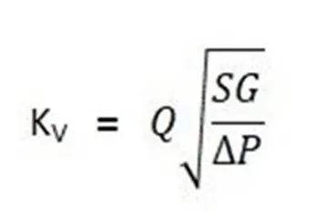

where,
Kv is the flow factor (expressed in m3·h−1).
Q is the flowrate (expressed in cubic metres per hour m3·h−1),
SG is the specific gravity of the fluid (for water = 1),
∆P is the differential pressure across the device (expressed in bar).
Kv can be calculated from Cv using the equation,

Solving & Modelling Approach -

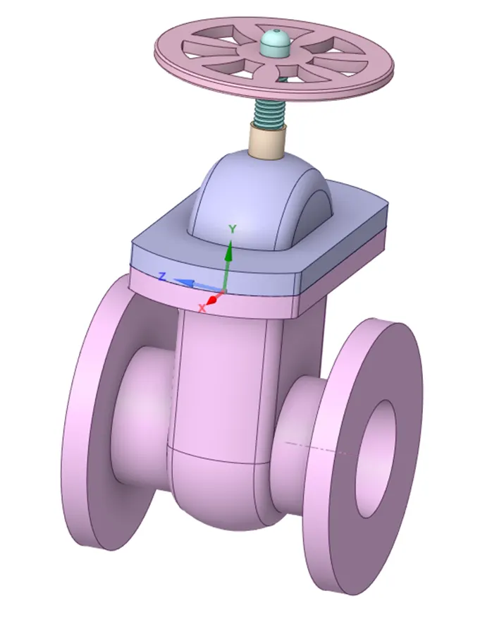
• Import the geometry in SpaceClaim
  
  Enabling Parameterization
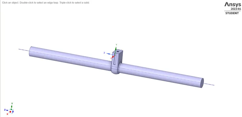
   Disable all solid parts besides the spindle and gate disc.
   Select the move option from the design tab, then move body from the drop-down menu, and finally gate disc. After seeing the coordinate system display on the gate disc, you can move the gate disc up towards the top of the spindle.

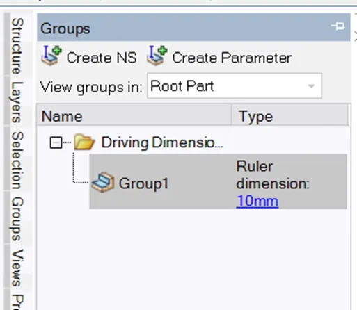
The alternative method to parametrize the lift dimensions, as shown in the image, is to navigate to the groups menu, which is next to the structured menu. There, you will be able to see the create parameter button, which will only be enabled after you have moved the gate disc. Click on create parameter, and then a group 1 will appear where you can edit the lift dimensions.Your gate disc lift will be parameterized as a result; you can verify this by looking at your workbench.

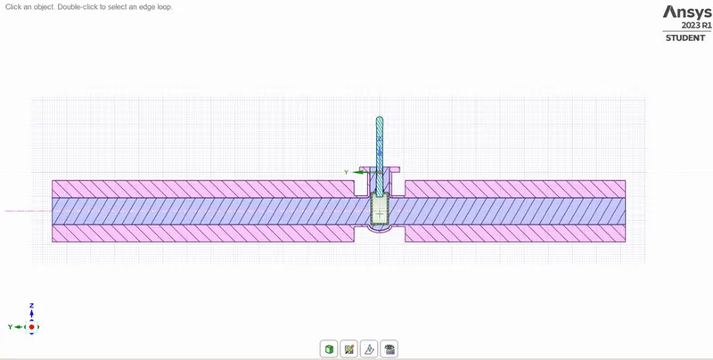
Verify the liquid volume. Whether it is correctly positioned relative to the disc.

Meshing –
• Activate the mesh console.
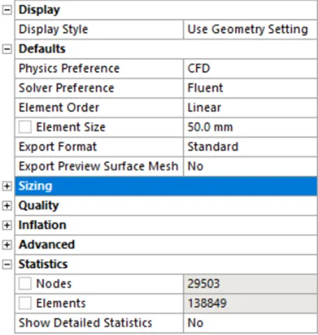
• Select the mesh element size 50mm for the mesh size and then click "generate mesh"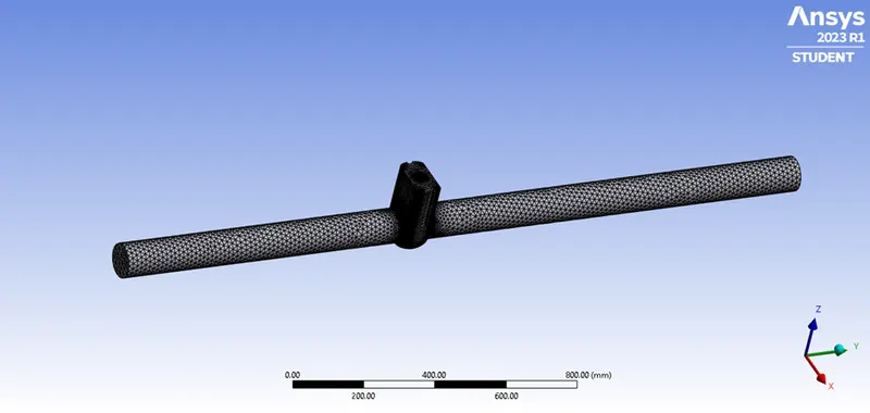

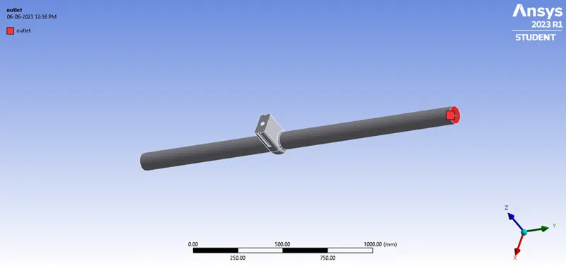
• For the inlet and outlet, create a named selection.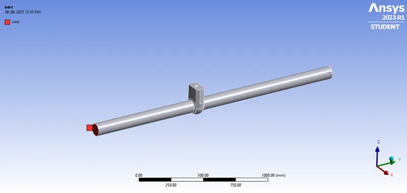


Total no. of elements:

Fluent Setup -

SOLVER TYPE	PRESSURE BASED
SOLVER TIME	STEADY STATE
GRAVITY	ON( Z AXIS AS -9.81m/s^2)
VISCOUS MODEL	K-EPSILON+REALIZABLE+SCALABLE WALL FUNCTIONS
MATERIAL	WATER
METHOD	COUPLED
INLET(PRESSURE INLET)	10 Pa
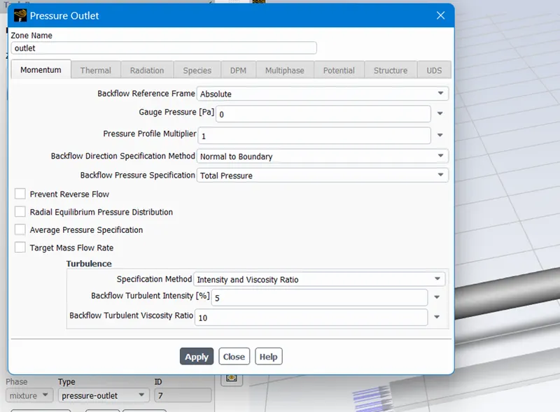
OUTLET PRESSURE	0 Pa

Carry out general setup, including enabling gravity and setting the solver time as steady state and pressure based.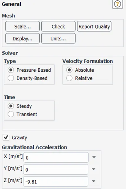

use viscous model as k-epsilon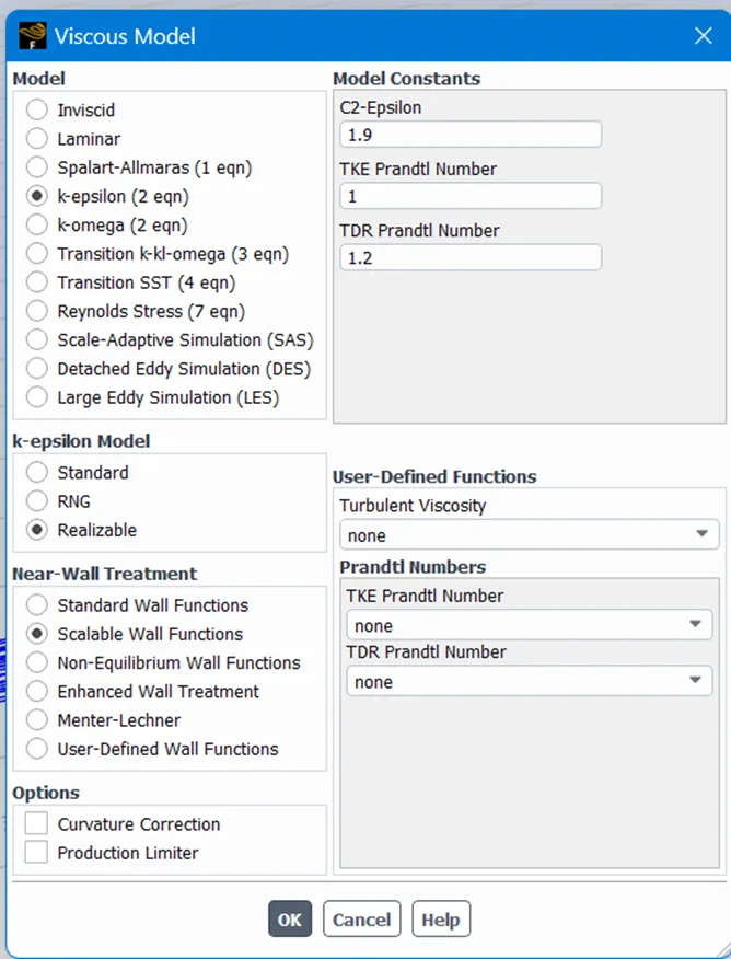

Using material as water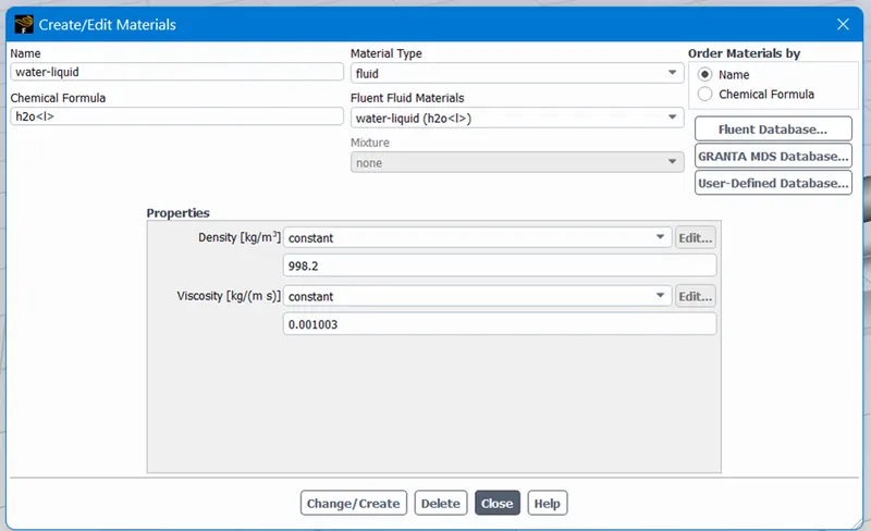

To display the findings in the project schematic window, create the plot for the mass flow rate at outflow and parametrize it.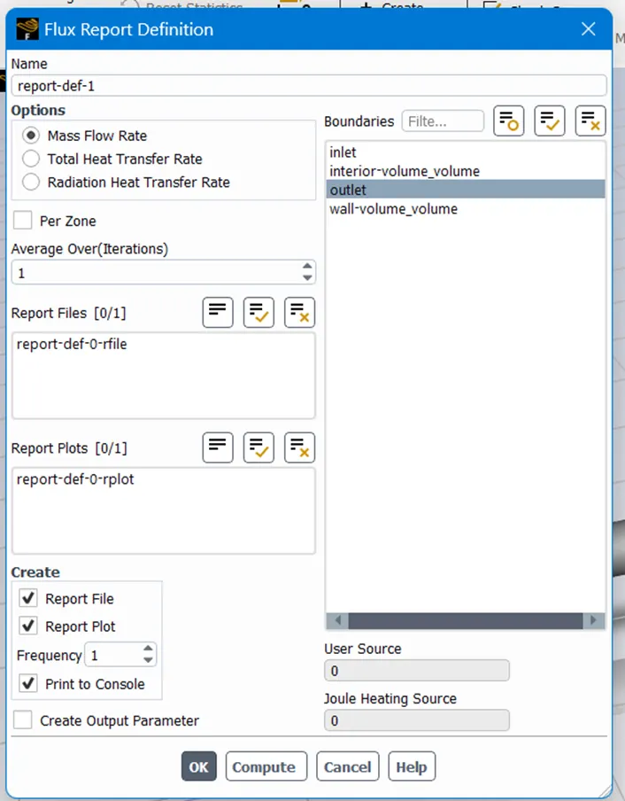

Make a plot for the outlet pressure and parametrize it.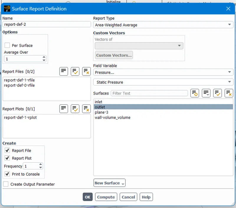

define the boundary parameters. pick the pressure inlet's inlet boundary.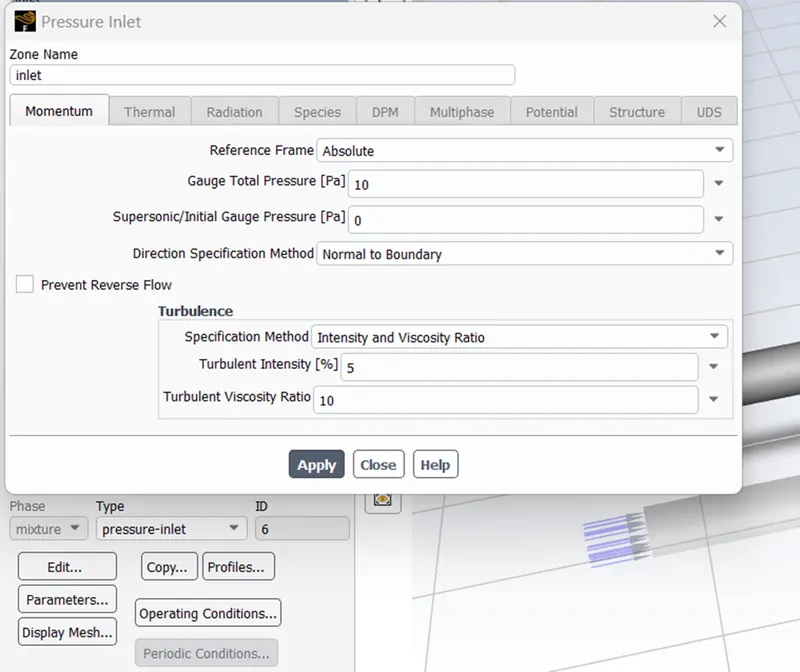

pick pressure outlet as the outlet boundary type.

initialize the problem using standard initialization.

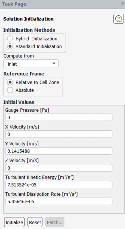
Run the simulation for 350 iterations.
Case 1: Gate Disc Opening is 10mm
• Scaled Residuals –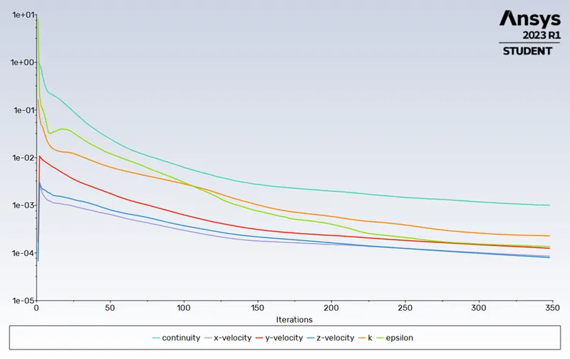

• Mass flow rate at outlet –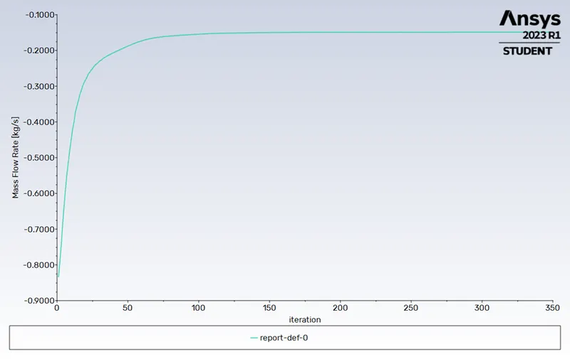

-0.14895604 [kg/s]
• Velocity Contours –

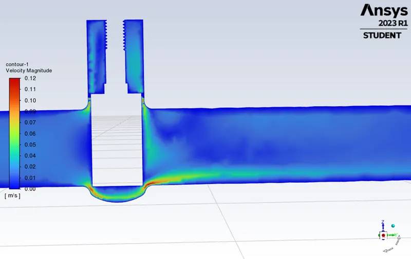
Case 2: Gate Disc Opening is 20mm
• Mass Flow Rate - -0.23839 [kg/s]
• Velocity Contours –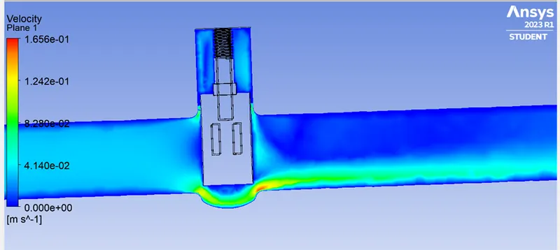

Next, we move on to the parameters tab to calculate the mass flow rates for the different wedge heights, and the following results were obtained,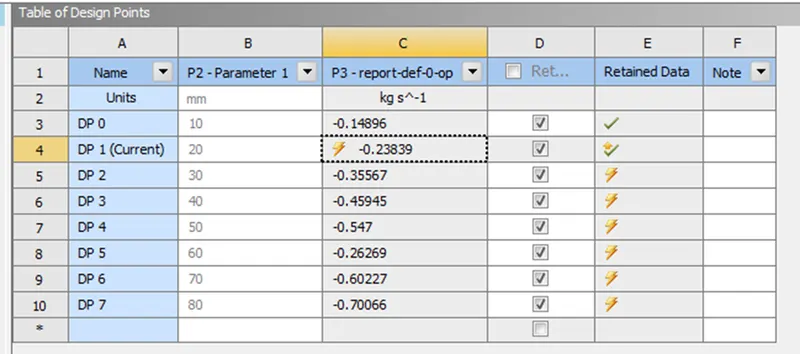

The negative signs for the mass flow rates imply that the fluid is exiting the domain. The mass flow rate is calculated for the stopper lifts from 10mm to 70mm. The mass flow rate increases with the increase in the lift of the stopper. When the stopper is lifted gradually, the space available for the passage of the fluid increases hence the mass flow increases. When we perform the parametric study, Ansys automatically changes the mesh as per new geometry using the same mesh specifications given earlier, and solves and calculates the output parameters, thereby saving time comparatively if it was done manually.
Magnitude of
Valve Displacement Mass Flow
Rate (Kg/s) Pressure
Outlet (Pa) Flow Factor (Kv) Flow Coefficient (Cv)
10 -0.14896 0.981 77.77 89.91
20 -0.23839 2.1651 128.53 148.59
30 -0.35567 3.7167 200.69 232.01
40 -0.45945 5.3669 273.47 316.15
50 -0.547 6.9184 344.35 398.09
60 -0.26269 8.5864 177.04 204.67
70 -0.60227 10.3864 442.27 511.30
80 -0.70066 12.4221 579.53 669.98
Results -

Magnitude of Valve Displacement	Mass Flow Rate (Kg/s)	Pressure Outlet (Pa)	Flow Factor (Kv)	Flow Coefficient (Cv)
10	-0.14896	0.981	77.77	89.91
20	-0.23839	2.1651	128.53	148.59
30	-0.35567	3.7167	200.69	232.01
40	-0.45945	5.3669	273.47	316.15
50	-0.547	6.9184	344.35	398.09
60	-0.26269	8.5864	177.04	204.67
70	-0.60227	10.3864	442.27	511.30
80	-0.70066	12.4221	579.53	669.98

Trend of Magnitude of valve displacement w.r.t. Kv & Cv

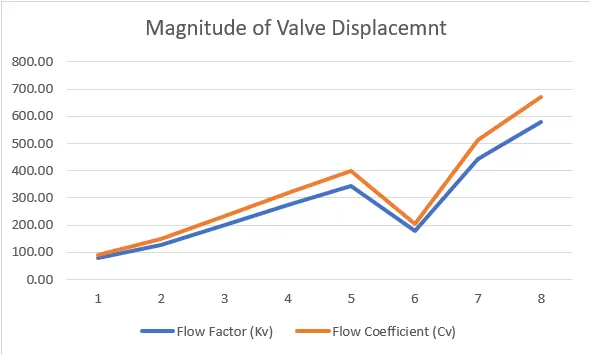
We may infer from the trend charts above that as the gate valve's opening grows, so does the mass flow rate. The flow factor and coefficient rise along with the mass flow rate.

Conclusion –
• You can define the parameter range, describe the design restrictions, and evaluate the effects of each parameter variation using parametric studies. You can assess your simulation once the settings have been generated. When you are happy with the outcomes, you can adjust the parameters or design limitations further.
• You can promote a configuration back to the model as a CAD edit if you've decided that it meets your design requirements. You are asked to update something. When doing simulations that call for repeating the same actions for several conditions, the parametric study method saves a tonne of time.
• In the parametric study of the gate valve, it was discovered that the flow factor and flow coefficient increase as the valve wedge is gradually raised, increasing the mass flow rate of the fluid.