Rayleigh Taylor Instability

Aim – To Conduct Rayleigh Taylor CFD Simulation.

Objectives –

• Explain different CFD models used for solving Rayleigh Taylor Instability problems
• Perform a Rayleigh Taylor instability analysis using the Volume of Fluid (VOF) multiphase model for air and water for two different mesh element sizes.
• Repeat the process for water and user-defined material with density = 400 kg/m3, viscosity = 0.001 kg/m-s, and compare the behaviour
• Define the Atwood number and derive it for each case. Explain the effect of Atwood number on instability.

So, there will be total of 3 cases

Case 1 : Mesh size- 0.5mm, Water and air

Case 2 : Mesh size- 0.1mm, Water and air

Case 3 : Mesh size- 0.1mm, Water and user defined fluid

Theory –

• Rayleigh-Taylor Instability

When the lighter fluid is pushing the heavier fluid, an instability known as the Rayleigh-Taylor instability, or RT instability, develops at the interface between the two fluids. Examples include how water behaves when it is suspended above oil in the gravitational field of Earth, mushroom clouds caused by volcanic eruptions and nuclear explosions in the atmosphere, supernova explosions in which the expanding core gas is accelerated into the denser shell gas, instability in plasma fusion reactors, and inertial confinement fusion.

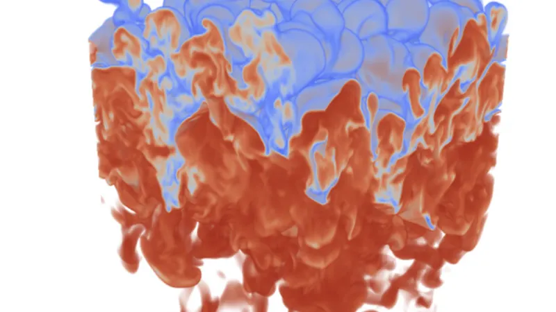
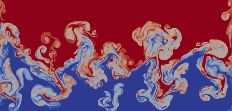
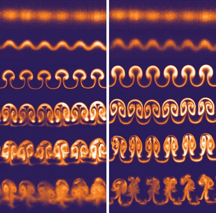
The initial perturbations evolve from a linear growth phase into a non-linear growth phase as the RT instability grows, eventually forming "plumes" that flow upward (in the sense of gravitational buoyancy) and "spikes" that fall below. The fluid flow can be closely approximated by linear equations during the linear phase, while the amplitude of perturbations increases exponentially over time. As a result, non-linear equations are needed to explain fluid motions in the non-linear phase since the change in amplitude is too great for a linear approximation. The structure of the following non-linear RT instability flows is often determined by the density disagreement between the fluids. (Assuming other variables such as surface tension and viscosity are negligible here). The Atwood number(A) is defined as the difference between the fluid densities divided by their combined value.

RT instability flows appear as symmetric "fingers" of fluid for A close to 0, whereas for A close to 1, the much lighter fluid "below" the heavier fluid appears as bigger bubble-like plumes.

This process can be seen in a number of examples on Earth, such as salt domes and weather inversions, as well as in astrophysics and electro hydrodynamics. For instance, the Crab Nebula, which is being cleaned up by an expanding pulsar wind nebula propelled by the Crab pulsar, exhibits RT instability structure. This supernova explosion occurred 1000 years ago. Recent research has also shown that the RT instability occurs when a relatively dense solar feature stands on top of a less dense plasma bubble in the solar corona, the Sun's outer atmosphere. The latter instance is comparable to RT instabilities with magnetic modulation.

• Stages of development and eventual evolution into turbulent mixing

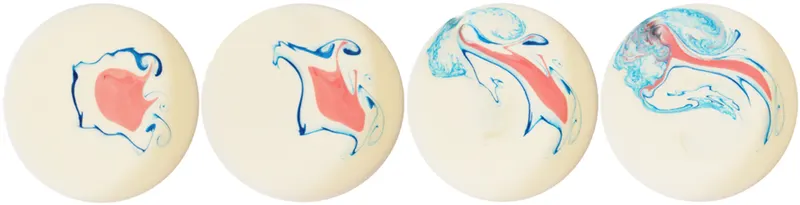
The RTI goes through four major stages as it develops. The motion equations can be linearized in the first stage when the disturbance amplitudes are tiny compared to their wavelengths, leading to exponential instability growth. A sinusoidal initial disturbance keeps its sinusoidal shape in the early part of this stage. However, following the conclusion of this initial phase, when non-linear effects start to manifest, one can see the beginnings of the construction of the typical mushroom-shaped spikes and bubbles (fluid structures of heavy fluid growing into light fluid). (Fluid structures of light fluid growing into heavy fluid).

The second stage of the mushroom structures' growth may be predicted using buoyancy drag theories, leading to a growth rate that is essentially constant throughout time. By this time, it is impossible to ignore the nonlinear elements in the equations of motion. The third stage then sees the bubbles and spikes start to interact. Bubble merging occurs when smaller bubbles and spikes combine to form larger ones due to the nonlinear interplay of mode coupling. Additionally, there is a bubble rivalry in which larger, less saturated bubbles and spikes surround smaller, saturated ones of a different wavelength.

This finally progresses to the fourth and last stage of the evolution, an area of chaotic mixing. If the Reynolds number is high enough, it is commonly believed that the mixing zone that eventually forms is self-similar and turbulent.

• Based on a mathematical understanding of RT waves, useful CFD models

1. Kelvin-Helmholtz instability
2. Richtmyer-Meshkov instability
3. Plateau-Rayleigh instability

1. Kelvin-Helmholtz instability

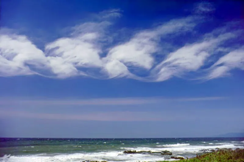
As well when there is a velocity variation across the interface between two fluids, this instability frequently arises when there is velocity shear in a single continuous fluid. The instability constant can be observed in waves on the water's surface as a result of wind blowing across it, which is a popular example. The Kelvin-Helmholtz instability is not just visible in clouds on water surfaces; it is also visible in the ocean and the sun's corona, among other natural phenomena. According to the hypothesis, fluids moving at varied speeds and with varying densities will eventually become unstable and change to turbulent flow. This instability happens when the interface of the two fluids experiences shear or a velocity differential.

2. Richtmyer-Meshkov instability

When two fluids with different densities are impulsively accelerated, this happens. Usually, a shock wave will pass through to do this. Small amplitude disturbances that first increase linearly with time are the beginning stages of the instability's development. After that, a nonlinear regime sets in, where bubbles occur when a light fluid penetrates a heavy fluid and spikes appear when a heavy fluid penetrates a light fluid. The two fluids eventually combine as a chaotic regime. This instability can be thought of as the Rayleigh Taylor instability's impulsive acceleration limit.

3. Plateau-Rayleigh instability

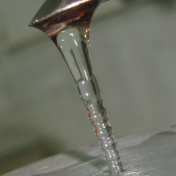
A falling stream of fluid breaks up into smaller packets with the same volume but less surface area because of this instability, which is frequently referred to as the Rayleigh instability. It is associated with RTI and belongs to a larger area of fluid dynamics that deals with fluid thread breaking. A specific kind of ink jet technology uses this fluid instability to its advantage by perturbing the liquid jet into a continuous spray of droplets. Liquids have a tendency to have smaller surface areas due to their surface tension, which is what causes the Plateau-Rayleigh instability.

• Atwood Number

When studying hydrodynamic instabilities in density stratified flows, fluid dynamics researchers utilise the Atwood number (A), a dimensionless quantity. A dimensionless density ratio is defined by,

Where,

ρ1= density of heavier fluid

ρ2= density of lighter fluid

Procedure –

• Geometry Preparation –

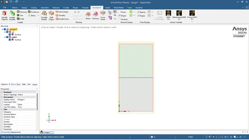
Open the space claim for geometry. For the two fluids, two 20x20mm squares are drawn one on top of the other. Once this is finished, the topology is shared, allowing for easy meshing.

When this procedure is finished. The space claim will be closed, and the mesh module will be opened.

Case 1 -

Mesh size - 0.5mm

Fluid - Water and air

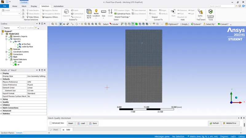
Open the mesh module, then select the CFD Fluent option and a 0.5mm element size under the mesh details. However, because this study will focus on mesh independence, a constant meshing size will be maintained throughout the volume. Take note of the study's nodes and elements count.

Check the quality requirement after the meshing is complete. Verify that the mesh quality is greater than 5%. After completing this, give the volume's faces the names "Water" and "Air."

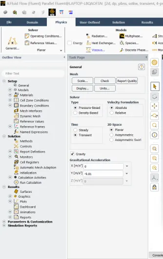
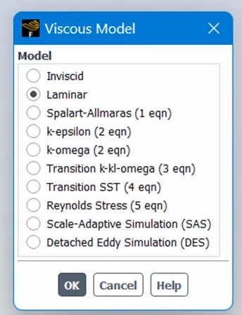
We must enter all the conditions, parameters, and models into ANSYS CFD. Go to the physics menu and select general settings to get started. Choose the Transient State Flow, Absolute Velocity Formulation, and Pressure Based Type Solver in that. Next, we must present the model. Laminar is chosen in this instance.

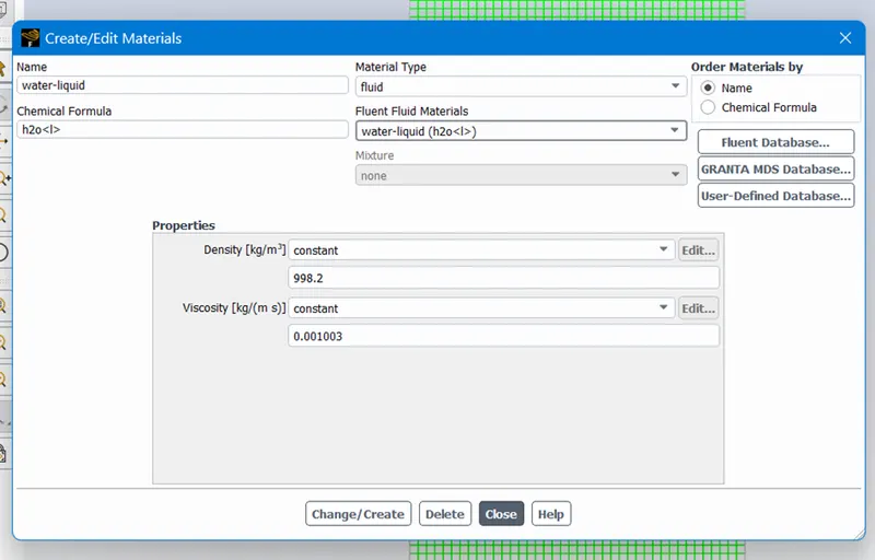
The choice of the flow material comes next. The default option is air. Two fluid phases exist. So choose water from the library of fluent words.

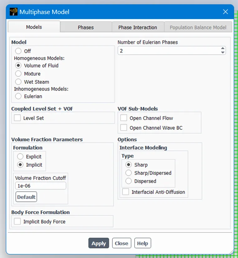
Select the volume of fluids with two fluids by clicking on the multiphase. Rename and allocate the major and secondary phases on the phases tab.

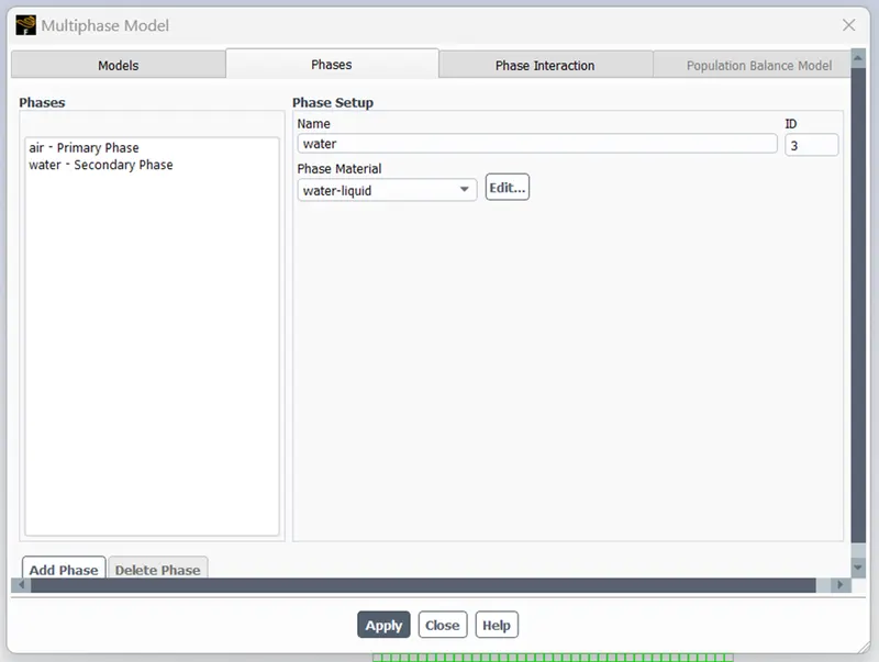
Move on to the solution section after the physics section is complete. Start by setting up the simulation. The boundary conditions are initialised by clicking Initialize. Initialization comes before the hybrid approach is chosen. To view an animation of the flow in the post results, select Autosave.

Patch the created region with the lubricating fluid. Set the fluid and select volume fraction. Set the values to 1 and 0.

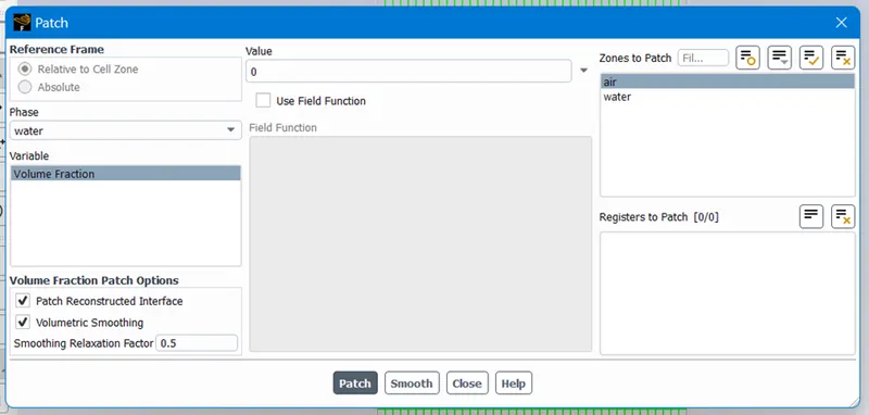
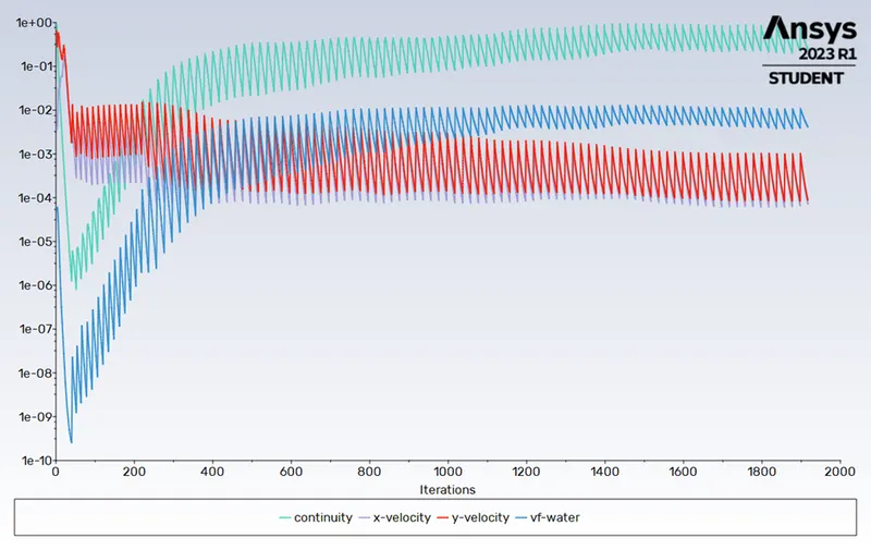
After then, repeat the calculation a certain number of times until convergence is reached. The amount of time needed for convergence varies depending on the model chosen and the number of elements. If necessary, we may calculate, measure, display, animate, etc. within the CFD module itself.

Results –

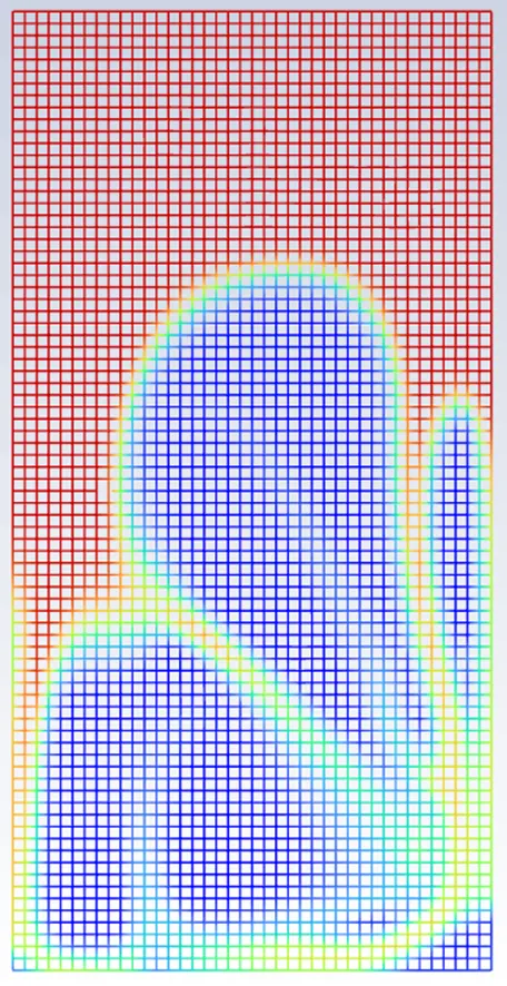
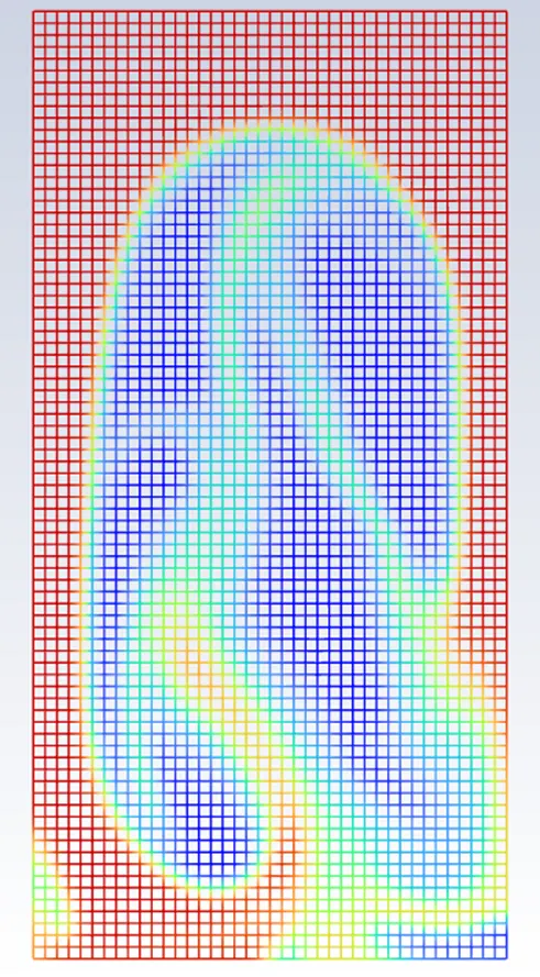
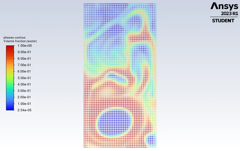
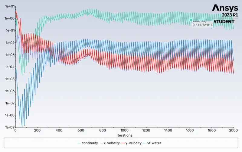
Click to watch Animation for Case-I

Case 2 -

Mesh size - 0.1mm

Fluid - Water and air

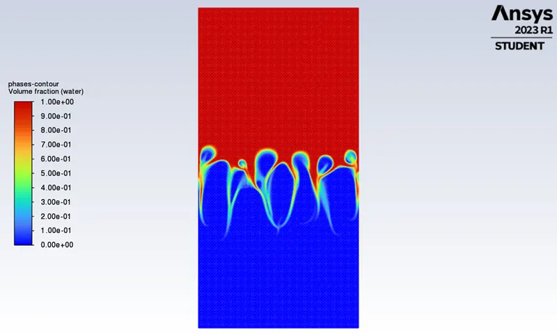
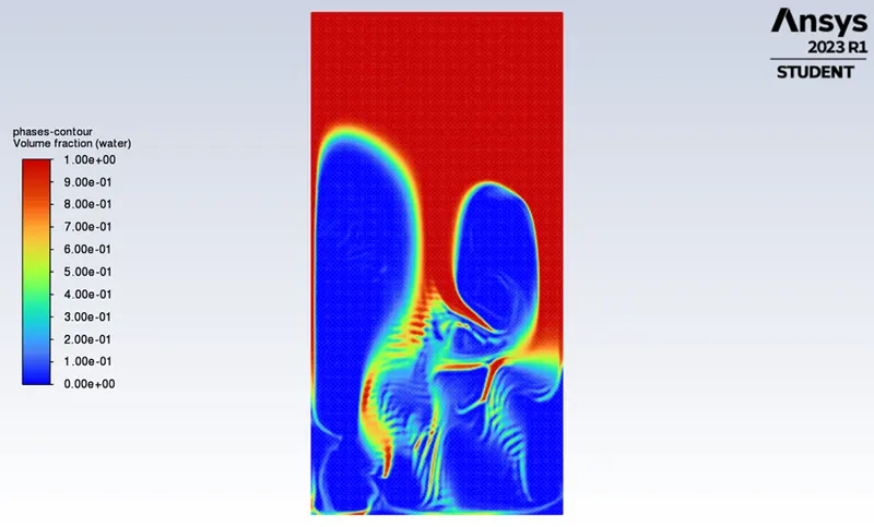
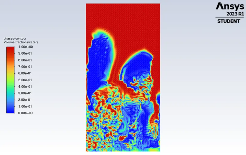
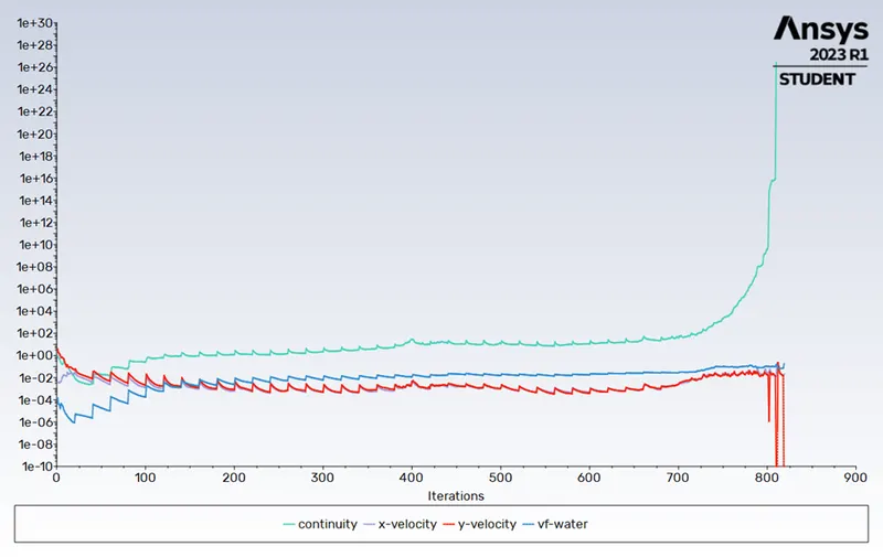
Click to watch Animation for Case-II

Case 3 -

Mesh size - 0.1mm

Fluid - Water and User Defined Fluid

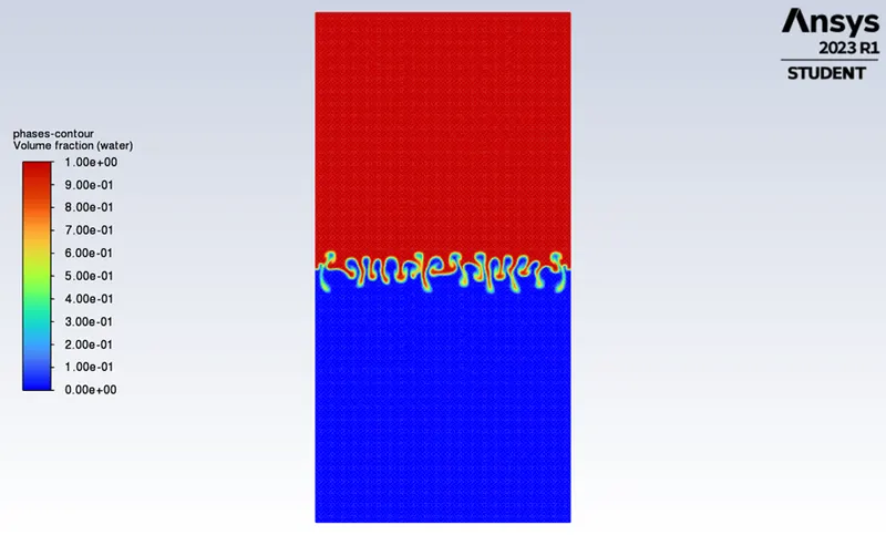
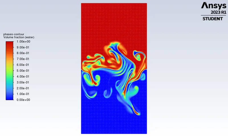
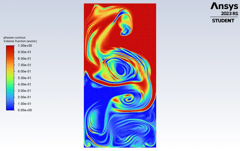
Click to watch Animation for Case-III

Atwood Number -

In order to explore hydrodynamic instabilities in density stratified flows, a dimensionless number is used which is nothing but the Atwood Number.

Where,

ρ1 is density of heavier fluid

ρ2 is density of lighter fluid

For Air-water RT instability,

ρ1 = 998.2 kg/m3 [Water density]

ρ2 = 1.225 kg/m3 [Air density]

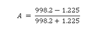
A = 0.998

For water- User Defined material RT instability,

ρ1 = 998.2 kg/m3 [Water density]

ρ2 = 400 kg/m3 [UD material density]

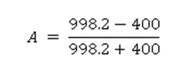
A = 0.428

Case no.	Fluids	Mesh Size	No. of Mesh Elements	Atwood No.
1	Air & Water	0.5	3200	0.9975
2	Air & Water	0.1	80000	0.9975
3	Water & User Defined Fluid	0.1		0.4278

Linear stability, mushroom head (falling or rising) or bubble (rising) generation, and long-term evolution as a result of bubble merging and mixing are the three distinct stages of RTI evolution. The bubble and mushroom head shapes are generally symmetrical for low Atwood numbers, and linear disturbances or perturbations last longer. The bubble and mushroom head shapes are less symmetrical and arise more quickly for big Atwood numbers, which results in a nonlinear growth rate. Although finer mesh better captures instability than coarse mesh, the heavier fluid takes longer to settle than fine mesh. Consequently, it costs more to compute but yields results that are more accurate.

Transient technique is favoured over steady state approach since the simulation requires capturing instabilities that change in an unanticipated way as a function of time.

Why Steady State simulation is not suitable ?

• We are aware that steady state simulation is a method that is independent of time.
• According to the simulation, there is significant turbulence present, and the flow changes over a very short period of time. In a steady state solution, this cannot be captured.
• Additionally, steady state solver ignores precisely capturing the simulation's non-linearities even though it may be able to capture the equilibrium state due to its disregard for the time differential factors included in the simulation.

Conclusion –

• From the examples mentioned above, we can see that a finer mesh catches instability better than a coarse mesh, but that the heavier fluid takes longer to settle than a fine mesh. Despite the lengthy computing time, the results are more accurate.
• The transient technique is favoured over the steady-state approach because the simulation must capture instabilities that change in an unanticipated way over time.
• The RT instability flows resemble symmetric fingers of fluid for Atwood numbers close to 0.
• The much lighter fluid beneath the heavier fluid manifests itself as larger bubble-like plumes when Atwood number approaches 1.

Click here to get Ansys Model