Simulation of Flow over a Cylinder.
Aim- To Simulate the flow over a cylinder and explaining the phenomenon of Karman vortex street.
PART-I
- Simulate the flow with the steady and unsteady case and calculate the Strouhal Number for Re= 100.
PART-II
- Calculate the coefficient of drag and lift over a cylinder by setting the Reynolds number to 10,100,1000,10000 & 100000. (Run with steady solver)
- Discuss the effect of Reynolds number on the coefficient of drag. [ Results should be validated with any standard literature and error should be within 5 %]
Theory-
- Flow Over Cylinder:
Even after nearly a century of rigorous experimental and numerical research, flow around a cylinder is still a difficult subject in fluid mechanics. In-depth studies are still being conducted to comprehend the intricate unsteady dynamics of the cylinder wake flow. Several engineering applications involve cross-flow that is normal to the axis of a stationary circular cylinder and the related issues with heat and mass transfer. Beyond a critical Reynolds number, experimental measurements and numerical calculations have both supported the onset of instability of the wake flow behind a cylinder, eventually leading to a type of periodic flow identified by distinct frequencies, popularly known as the Von Karman vortex street in the literature.
Laminar flow past cylinders with regular polygonal cross sections typically separates at one or more sharp corners of the geometry of the cross section itself, leaving a system of vortices on either side of the mid symmetry plane in the aftermath. On the other hand, the mechanics of the flow are far more complicated than what its deceptively simple shape may imply for a circular cylinder, where the point of flow separation is determined by the makeup of the upstream boundary layer.
- Strouhal Number
The Strouhal number, which describes oscillating flow mechanisms, is a dimensionless number used in dimensional analysis.
Viscosity predominates fluid flow at high Strouhal numbers (order of 1), causing the fluid "plug" to collectively oscillate. The high-speed, quasi-steady-state component of the movement dominates the oscillation for low Strouhal numbers (order of 10-4 and lower). Vortex accumulation and swift vortex shedding are characteristics of oscillation at intermediate Strouhal numbers.
Frequently, the Strouhal number is stated as,
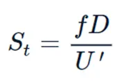
Where,
f= frequency of vortex shedding
D= characteristic diameter of the cylinder
U'= fluid flow velocity
- Coefficient of Drag
The drag coefficient, which has no dimensions and is employed in fluid dynamics, is a measurement of an object's drag or resistance in a fluid environment like air or water. It is utilised in the drag equation, where a lower drag coefficient denotes a reduced aerodynamic or hydrodynamic drag for the item. A specific surface area is constantly linked to the drag coefficient.
Each object's drag coefficient combines the effects of form drag and skin friction, the two primary causes of fluid dynamic drag. The effects of lift-induced drag are also included in the drag coefficient of a lifting airfoil or hydrofoil. A full structure, like an aircraft, has a drag coefficient that takes interference drag into account as well.
The drag coefficient (Cd) is defined as,
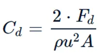
Where,
Fd = drag force, which is by definition the force component in the direction of the flow velocity
ρ = mass density of the fluid
u = flow speed of the object relative to the fluid
A = reference area
4. Coefficient of lift
A lifting body's lift is related to the fluid density, fluid velocity, and a related reference area through the lift coefficient, which is a dimensionless coefficient. A fixed-wing aeroplane is an example of a lifting body, as is a foil or a whole foil-bearing body. CL depends on the body's Mach number, Reynolds number, and angle to the flow. The section lift coefficient cl refers to the dynamic lift characteristics of a two-dimensional foil section, with the reference area substituted by the foil chord.
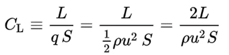
Where,
L = Lifting Force
S = Relevant Surface Area
q = Fluid Dynamic Pressure
Procedure for geometry -
To create the geometry we need to open SpaceClaim from ANSYS workbench. After opening SpaceClaim we need to draw geometry from the Y-axis which is circle of 2 meter dia.
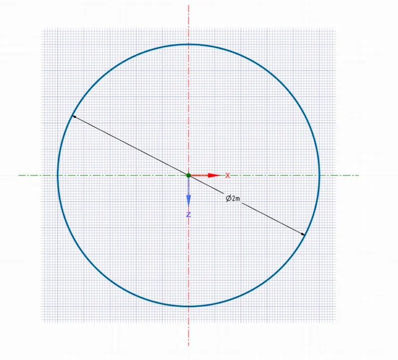
After drawing circle from sketch mode, we need to create computational domain as given in video. Which is of 10 times the diameter i.e.., 20m distance from the geometry and the outlet boundary will at 40m. Also the inlet will be of 0.5 times the diameter i.e.., 10m from each side.
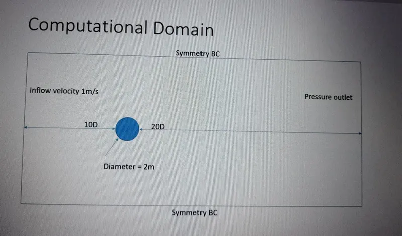
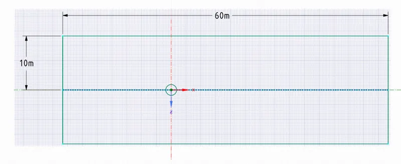
To convert it into surface we need to use the pull tool, which converts sketch into the surface.
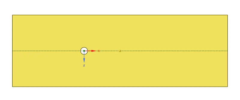
This completes the geometry creation process.
Then in next step generate the mesh with 2m element size and triangular type of elements.
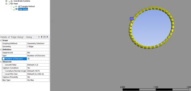
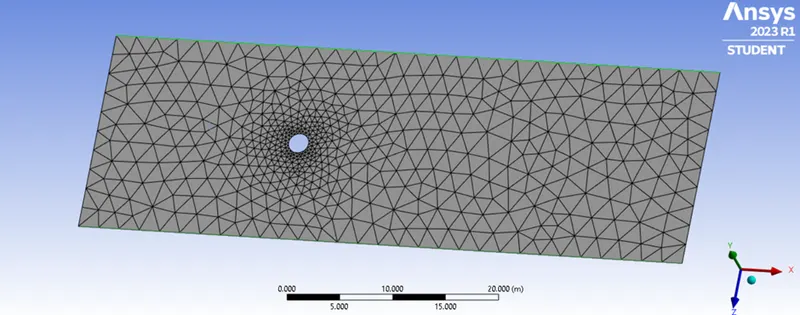
Now moving to setup,
At first we check the mesh. Then physics parameters as shown in below figure,
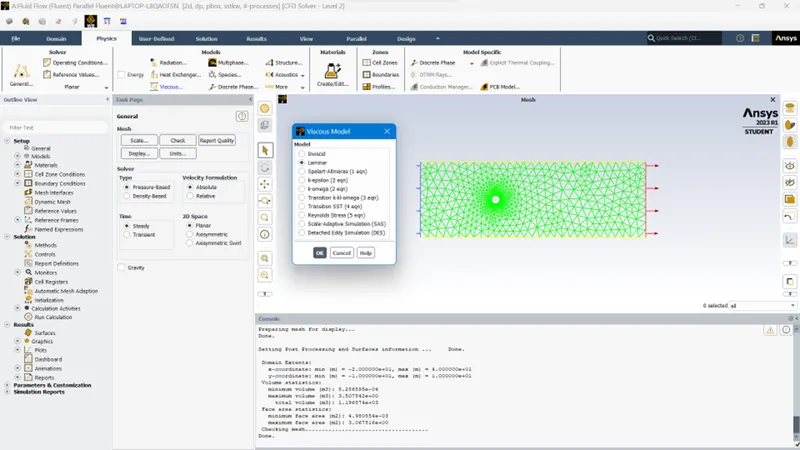
We are controlling the Reynold’s number by modifying the dynamic viscosity. Then the assign the material i.e. Air
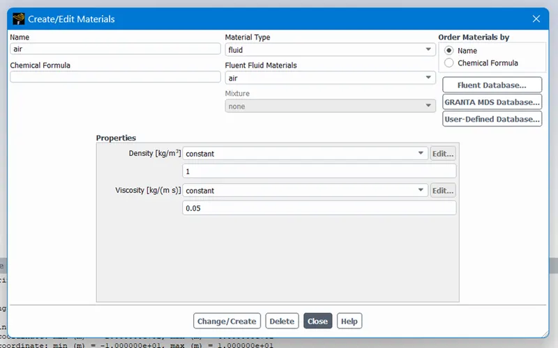
Check to see if the fluid is updated by opening Zones and entering the inlet velocity in accordance with Reynolds' number.
Change the reference values in the setup area's right-hand section.
Also create a monitor-point using create command
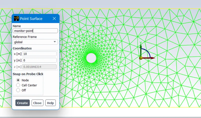
Fluent procedure/details:
- Laminar model,
- fluid is air.
- Basic discretization technique
- Kinematic viscosity/density: 1/0.05
- By selecting point under surfaces in the results bar, creating a monitor point behind the cylinder.
- Create reports or charts for drag, lift, and velocity relative to the cylinder after creating the monitor point.
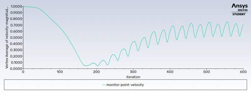
- To study the vortex shedding, plot the velocity at the monitor point.
- For steady-state and transient state simulations, use hybrid initialization.
PART-I
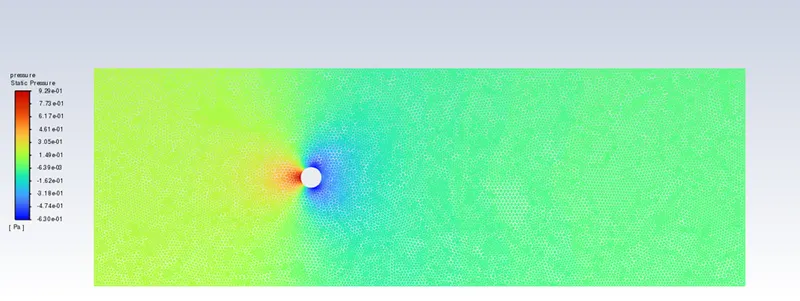
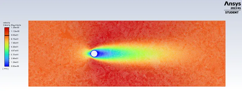
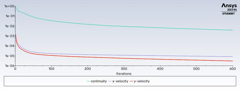
(i) Simulation of the flow with the steady case and calculate the Strouhal number for Re=100 and velocity 1m/s.
- Pressure Contours
- Velocity Contours
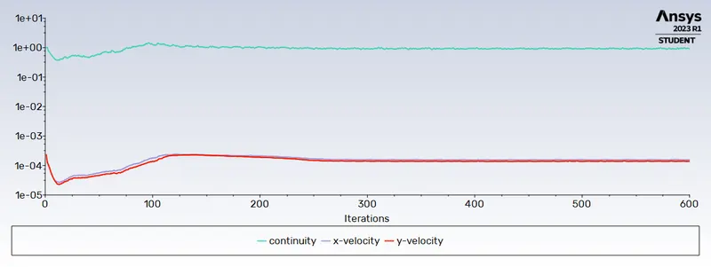
- Residuals Plots
- Monitor Point Velocity
- Strouhal Number
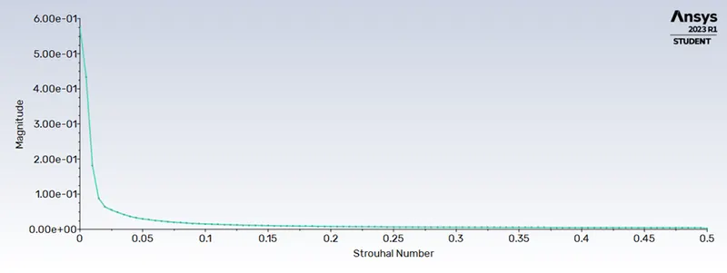
(ii) Simulation of the flow with the unsteady case and calculate the Strouhal number for Re=100 and velocity 1m/s.
- Pressure Contours
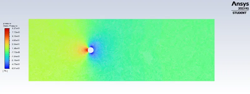
- Velocity Contours
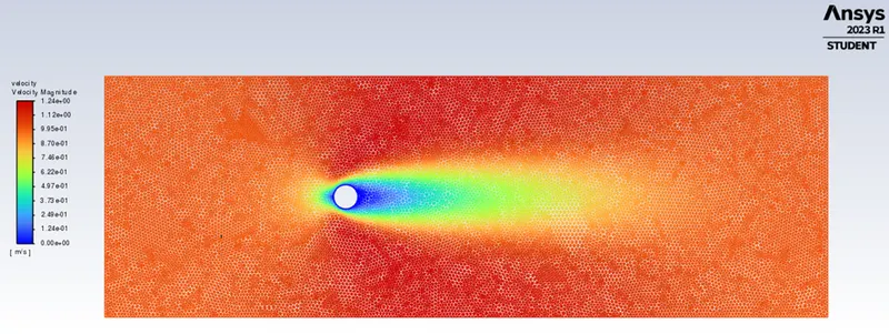
- Residual Plots
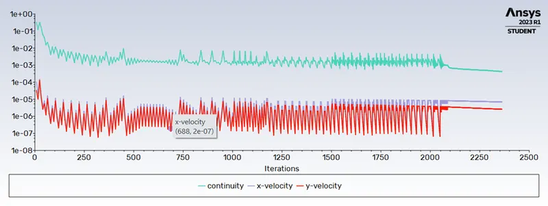
- Monitor-Point Velocity
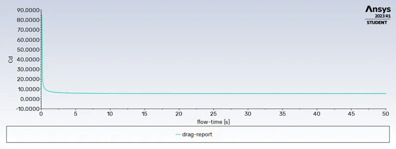
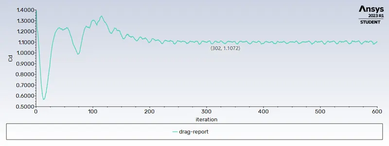
- Drag Report
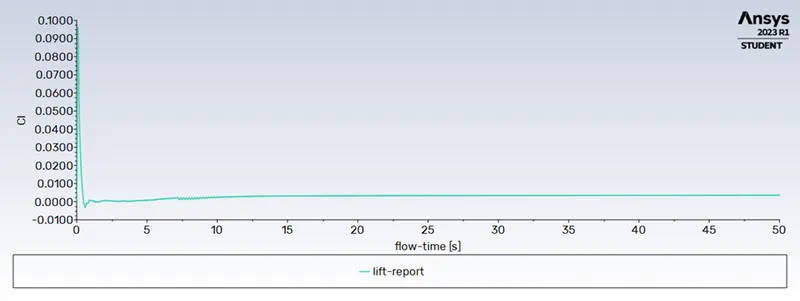
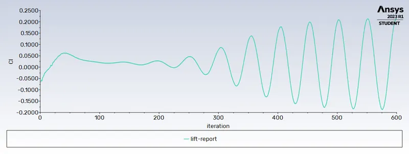
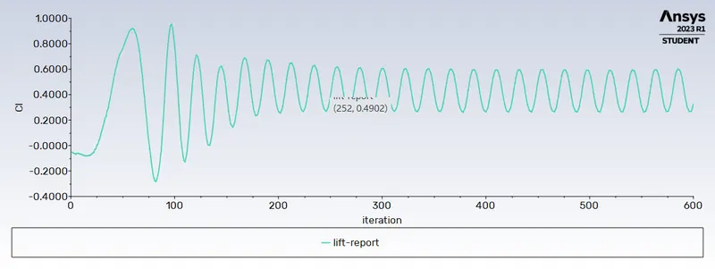
- Lift Report
- Strouhal Number
PART-II
(i) Simulation of the flow with the steady case and calculate the Strouhal number for Re=10 and velocity 1m/s.
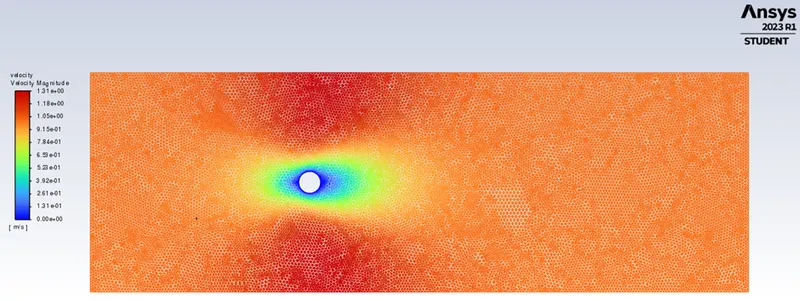
- Velocity Contours
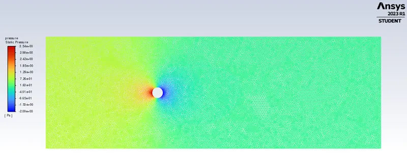
- Pressure Contours
- Residual Plots
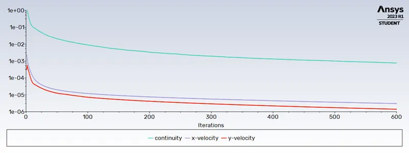
- Drag Report
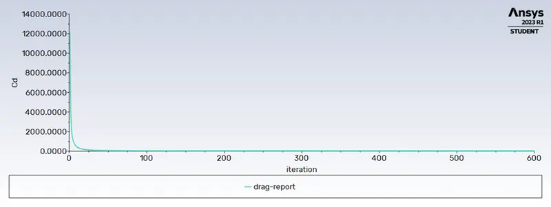
- Lift Report
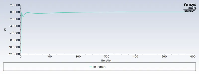
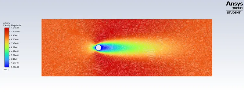
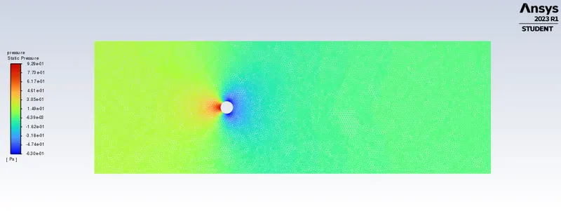
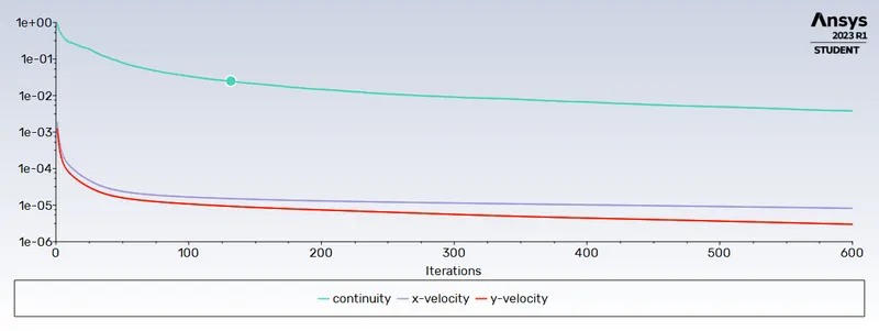
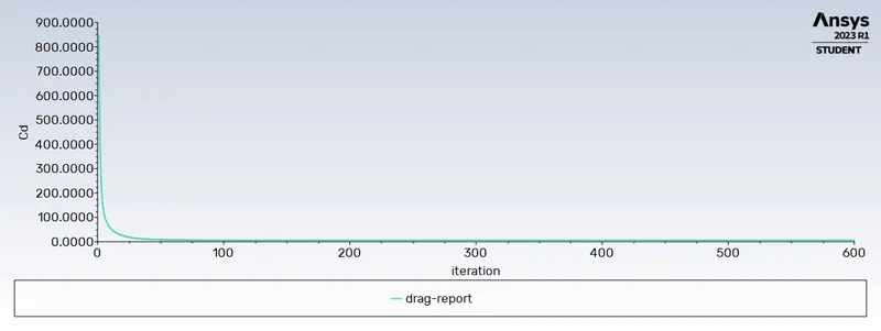
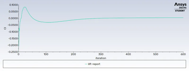
(ii) Simulation of the flow with the steady case and calculate the Strouhal number for Re=100 and velocity 1m/s.
viscosity=0.2
- Velocity Contours
- Pressure Contours
- Residual Plots
- Drag Report
- Lift Report
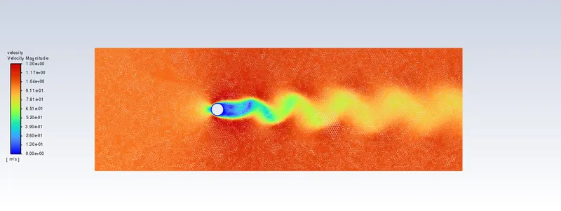
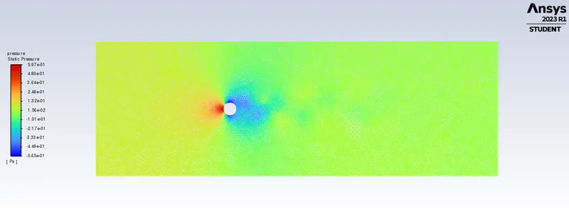
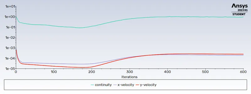
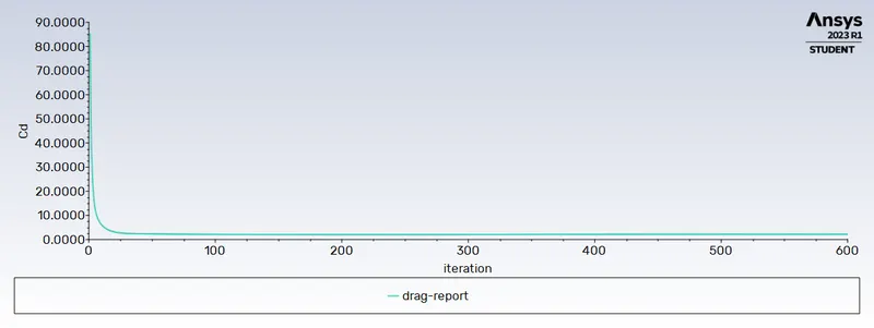
(iii) Simulation of the flow with the steady case and calculate the Strouhal number for Re=1000 and velocity 1m/s.
viscosity=0.02
- Velocity Contours
- Pressure Contours
- Residual Plots
- Drag Report
- Lift Report
(iv) Simulation of the flow with the steady case and calculate the Strouhal number for Re=10000 and velocity 1m/s.
viscosity=0.002
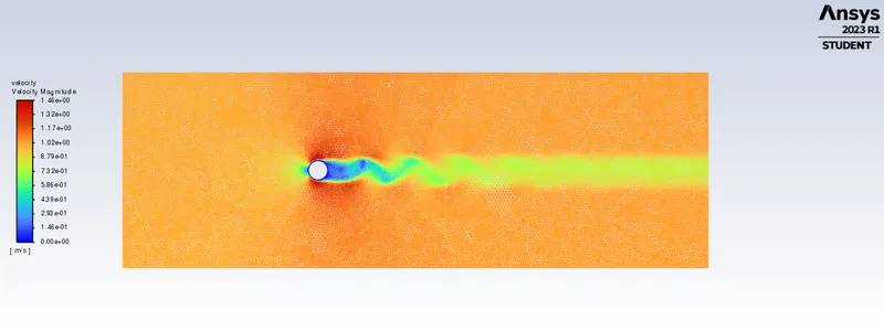
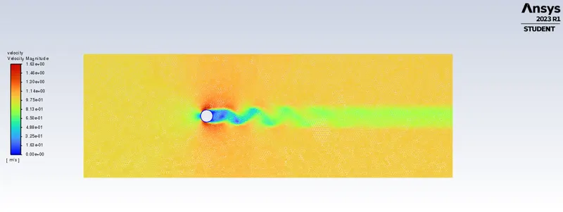
- Velocity Contours
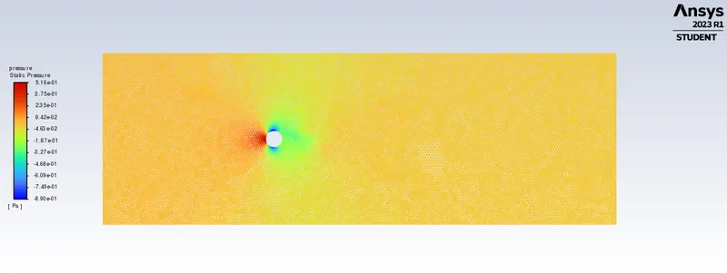
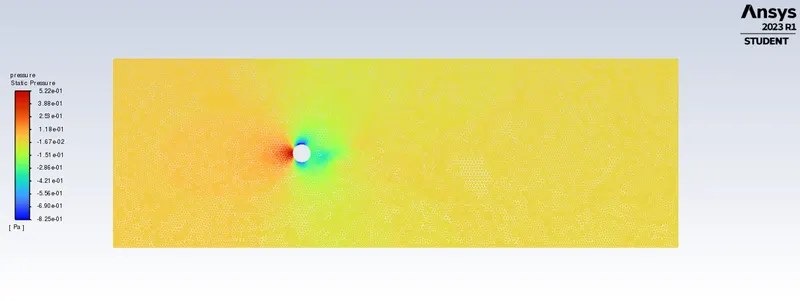
- Pressure Contours
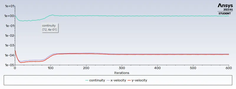
- Residual Plots
- Drag Report
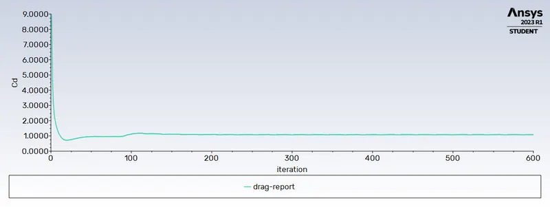
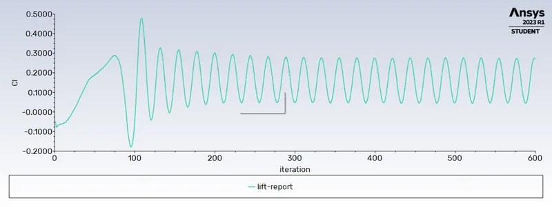
- Lift Report
(v) Simulation of the flow with the steady case and calculate the Strouhal number for Re=100000 and velocity 1m/s.
- Velocity Contours
- Pressure Contours
- Residual Plots
- Drag Report
- Lift Report
Result -
| Re | Cd">Cd (Drag) | CL">Cl (Lift) |
| 10 | 3.39 | -0.00135 |
| 100 | 1.367 | -0.11 |
| 1000 | 0.856 | -0.00843 |
| 10000 | 0.9883 | -0.376 |
| 100000 | 0.943 | 0.878 |
Effect of Reynolds number on the coefficient of drag i.e.., Error with respect to the theoretical values from the reference material,
| Reynolds number | theoretical Cd | Numerical Cd | error |
| 10 | 3.5 | 3.39 | 3.14% |
| 100 | 1.4 | 1.367 | 2.36% |
Conclusion -
- The flow across a cylinder is simulated in the first instance for both steady and unstable scenarios with Re=100, and from the results, the Von Karman Vortex Street phenomenon is also seen.
- Plots that are necessary to see that the flow has converged and that vortex shedding is occurring are created.
- It is possible to determine the Strouhal number by plotting Power Spectral Density vs. Frequency.
- In the second scenario, six distinct simulations, with Reynolds numbers of 10, 100, 1000, 10000, 100000, and 1000000, are run to observe how the drag and lift coefficients behave.
- The Reynolds number is changed by varying the flow velocity while holding the other parameters constant in order to study how the drag coefficients behave in the simulations.
- The creation of vortex shedding is not detected for Re=10, but it is clearly shown in the other situations.
- The mistake percentage is less than 5%, according to the above table.