External flow simulation over an Ahmed body.

Aim-

To perform external aerodynamic simulation over Ahmed-body

Objectives-

1. To determine the aerodynamic forces on the Ahmed body i.e., Drag & Lift Force
2. To Perform Grid Dependency Test

Theory –

• Ahmed-Body -

The Ahmed body is a generic car body (a simple vehicle model). The airflow around the Ahmed body captures the essential flow features around an automobile and was first defined and characterised in the experimental work of SR Ahmed in his research Some noteworthy elements of time average ground vehicle wake. Although it has a very simple shape, the Ahmed body allows us to capture characteristic features that are relevant to bodies in the automobile industry.

This model is also used to represent the turbulent flow field around a car-like geometry. New car models are created using the numerical model after it has been found to be inaccurate. The rear part of Ahmed's body called as 'slant angle' which influences drag and lift with its critical slant angle which is around 0-30 degrees.

It is used for testing new CFD solvers or testing one's ability to perform simulations as there is a plethora of experimental data available about the Ahmed body to compare simulation data to.

Besides the analyses of the velocity field, the Ahmed Body is also used for drag force and lift force analyses and rolling, pitching and yawing moments. The slant angle on the back permits examining the separation zone and its influence on the velocity profile and forces.

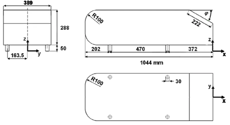
The geometry of the Ahmed body is shown in the figure below. The slant angle is adjustable and is the main variable model parameters in the experimental investigations. The Ahmed body, of length (L) 1044 mm, height (H) 288 mm, and width (W) 389 mm, was placed at 50 mm from the ground (G).

• The Y+ Concept -

As any viscous flow flows across a surface, a zone of slow-moving flow termed the boundary layer emerges. There is a significant velocity gradient and nonlinear variation of U inside the boundary layer. It is important to distinguish these layers to model the boundary physics correctly and use an appropriate turbulence model. Hence, Y+ is a non-dimensional distance normal from the wall. It is applicable to all flows.

For a CFD simulation, we can compute the first layer height for a desired Y+ value with the following formula

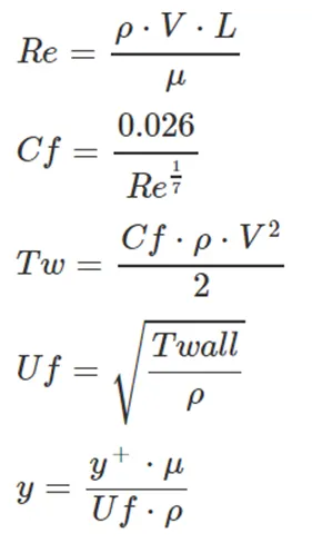
Where,

ρ is fluid density ;

µ is fluid viscosity ;

U is the free stream velocity ;

L is characteristic length ;

Uτ is frictional velocity ;

τω is wall stress ;

Cf is the skin friction coefficient

• Boundary Layer -

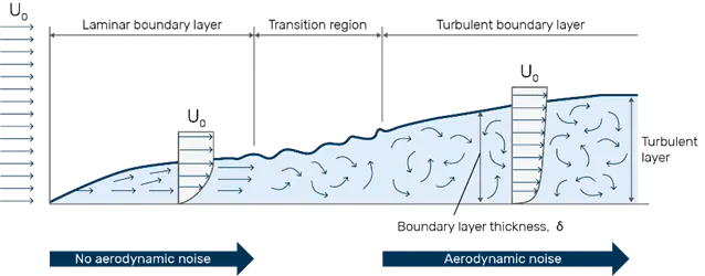
A boundary layer is a thin layer of true fluid along the surface of an object whose viscosity affects the fluid dynamics. As the liquid flows across the plate, the velocity is much lower near the surface, creating turbulence.

In the no-slip condition, the relative velocity at the disk is assumed to be zero and continues to increase until the free stream velocity is reached. The boundary layer thickness increases with the length of the plate.

In the narrow boundary layer adjacent to the plate, shear and inertial forces are equally important in determining the motion of fluid elements, and out-of-domain shear stress can be neglected. Liquid deceleration is transferred from one liquid layer to another by viscosity, forming a velocity gradient in the boundary layer. Boundary layer thickness is often described as the distance from the plate until the velocity reaches 99% of the free stream velocity.

The velocity gradient (∂u/∂y) normal to the wall multiplied by the viscosity (μ) is the wall friction or shear stress. The greater the velocity gradient perpendicular to the wall, the greater the shear stress.

As the velocity gradient along the flow direction decreases, so does the shear stress. The increase in boundary layer thickness along the plate can be explained by considering the temporal evolution of the vorticity within the boundary layer.

Viscosity acts via a molecular diffusion mechanism to propagate eddies as they convict downstream. The local boundary layer thickness is a measure of the distance of the eddy that has diffused away from the plate.

Since we are dealing with turbulent boundary layers and related phenomena, we do not want to deal with laminar boundary layers. The figure above shows that in the turbulent boundary layer domain, the near-wall flow is solved in three layers. Inner or sublayer (viscous shear dominates) Outer or defect layer (largely turbulent eddy shear dominates) Overlap or logarithmic layer (velocity profile exhibits logarithmic variation).

• Flow Separation -

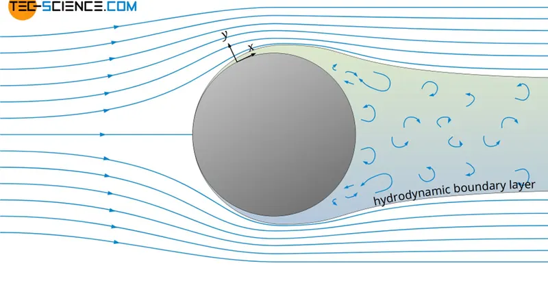
When a liquid flows at high speed over a curved surface. Liquid follows easily the front part of the curved surface, but does not easily adhere to the rear part.

At sufficiently high velocities, the liquid stream leaves the surface of the body. This is called flow separation.

The location of the detachment point depends on several factors such as Reynolds number, surface roughness and degree of free-stream fluctuation. It is usually difficult to predict exactly where delamination will occur unless there are sharp corners or abrupt changes in shape. solid surface. This contributes to the formation of pressure drag that affects vehicle performance.

Importance of Ahmed Body –

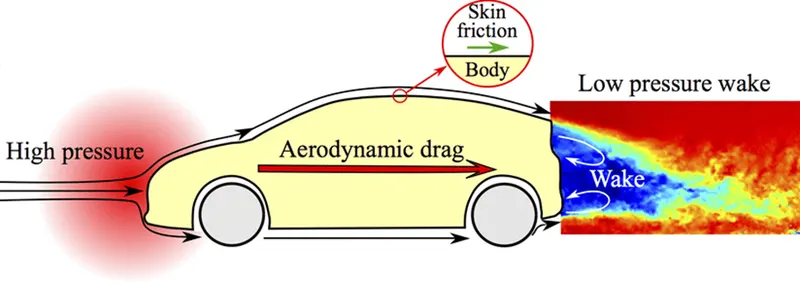
The Ahmed body generates the crucial features of flow pattern around a car for instance flow impinge-mentation and the displacement around the nose, relative uniform flow of air around the middle portion and flow separation along with the wake generation at the rear. Since the Ahmed body is easy to model, it can be effortlessly utilized for researching various properties like turbulence, drag coefficient, wake region, lift forces, velocity magnitude at various regions of the car, magnitude of pressure around the car which helps in determining what will be resistance, fuel efficiency etc. of the car thereby providing designers a clear idea on which region needs to be optimized for better effectiveness.

Negative Pressure in Wake Region –

The wake is a sizable low-pressure turbulent zone that is left behind a vehicle when the air travelling over it is split at the back end. This wake helps create pressure drag, which eventually lowers the performance of the vehicle.

The area of recirculating flow immediately after a moving or stationary blunt body, caused by viscosity, which may be accompanied by flow separation and turbulence flow, or the pattern of waves on the water's surface produced by a moving object (such as a ship), caused by density differences of the fluids above and below the free surface and gravity.

The viscous effects in the fluid are contained within a small layer known as the boundary layer while the vehicle is travelling at a specific velocity. The inviscid flow is found outside of the boundary layer. The boundary layer is under pressure due to this fluid flow. The fluid becomes dislodged when air enters the vehicle's rear. The viscosity effects of the fluid completely control how the fluid moves within the boundary layer. The Reynolds number is influenced by the vehicle's characteristic length, kinematic viscosity, and speed. The fluid's ability to circulate around a vehicle is influenced by its shape and Reynolds number.

Another significant occurrence also has an impact on the performance and flow of the vehicles. This occurrence is frequently referred to as the vehicle "Waking." The wake is a sizable low-pressure turbulent zone that forms when the air flowing over the vehicle is split at the rear end. This wake helps create pressure drag, which eventually lowers the performance of the vehicle.

Procedure –

• Importing Ahmed -Body Geometry -

• Splitting body into half -

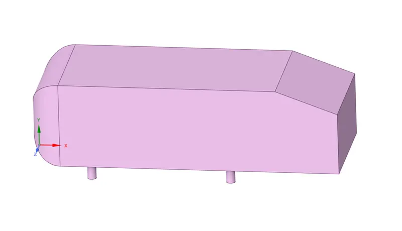
Since this is a complex simulation and the Ahmed body is symmetrical along the z axis, the geometry was split into two along the z axis using ANSYS's split tool.

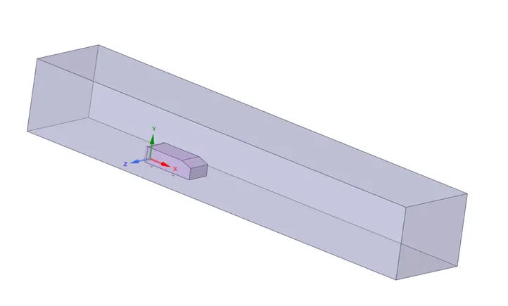
• Creating an Enclosure -

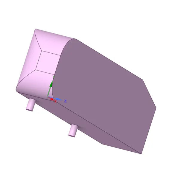
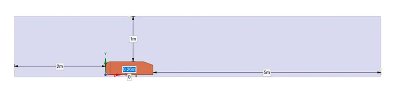
As we are simulating flow outside the Ahmed-Body we need to create an outside body i.e.., An Enclosure by using Enclosure command in SpaceClaim.

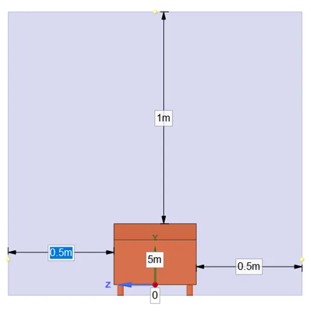
The Dimensions of the Enclosure is as follow:

• Mesh Generation -

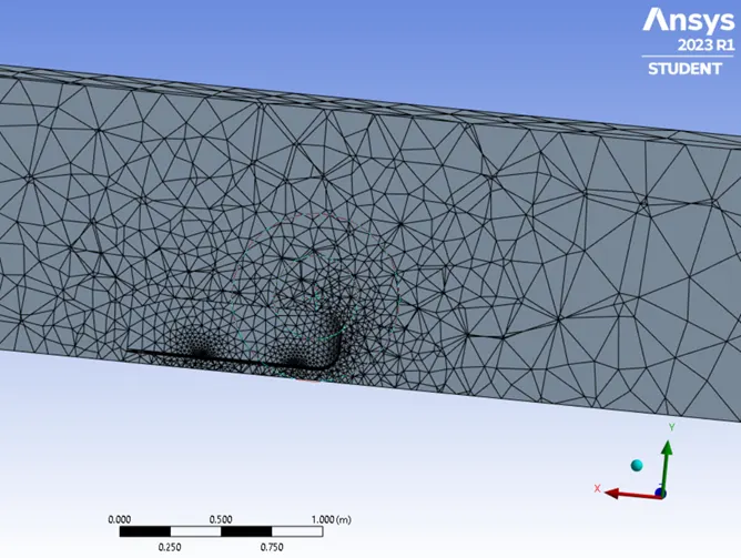
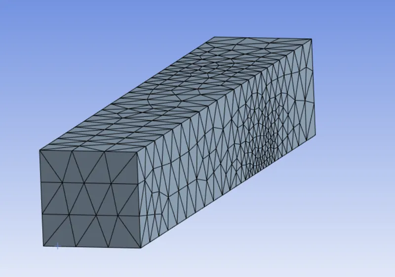
At first we are generating only base mesh with all the default values to see that everything is fine.

• Setup -

As we are running this simulation for air velocity of 25m/s which is much less for Mach number and also we are supposed to get good compressibility effects, That’s why we are using Density-Based Solver.

The reason for choosing Steady state time is to calculate different drag forces, velocity distribution, etc.

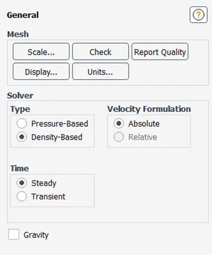
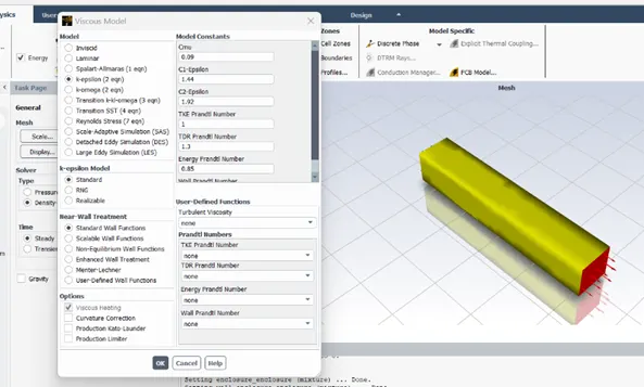
We are choosing K-epsilon model for solving and also we are turning on energy equation.

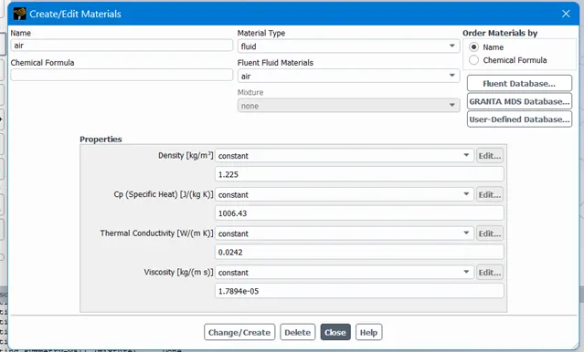
We are choosing default material setting for Air.

This completes Setup.

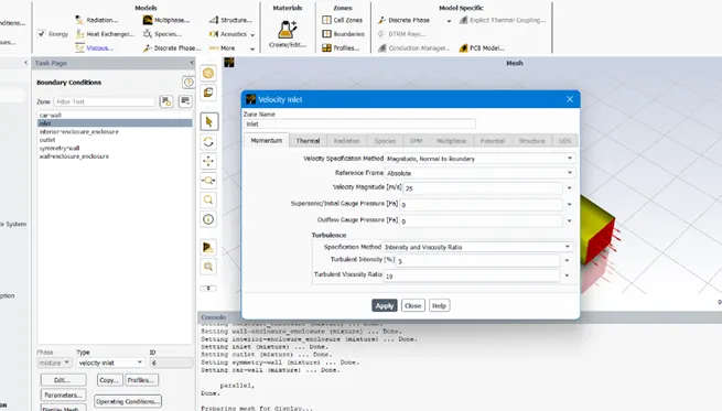
Now the boundary conditions,

• Results -

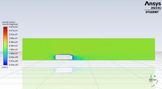
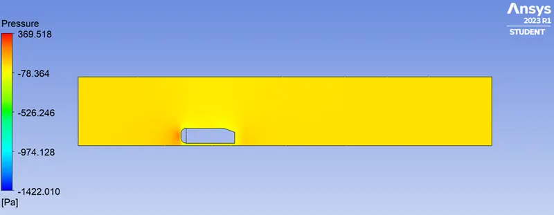
1.Velocity and Pressure Contours

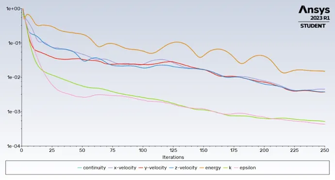
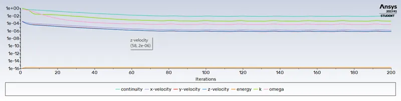
2. Scaled Residuals

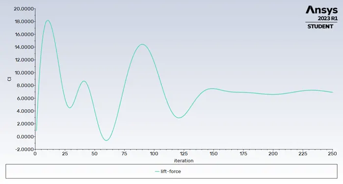
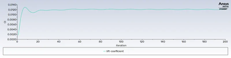
3. Lift Force

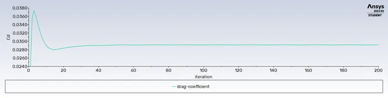
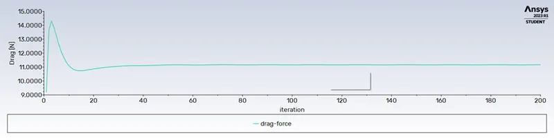
4. Drag Force

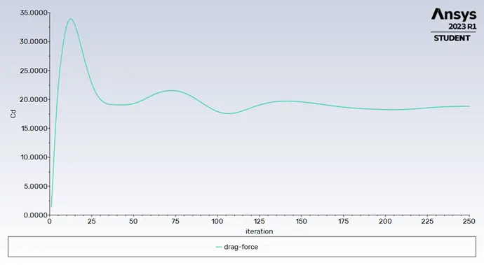
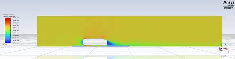
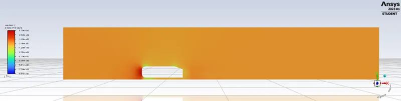
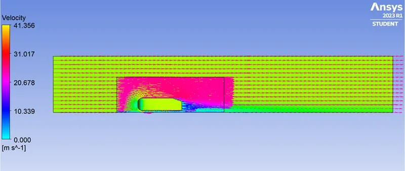
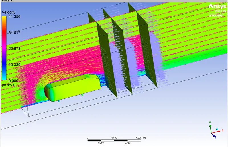
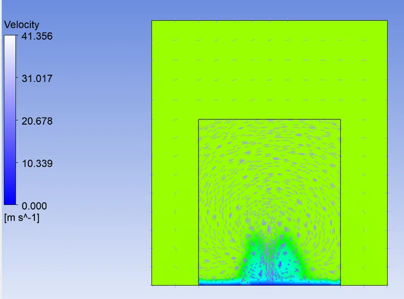
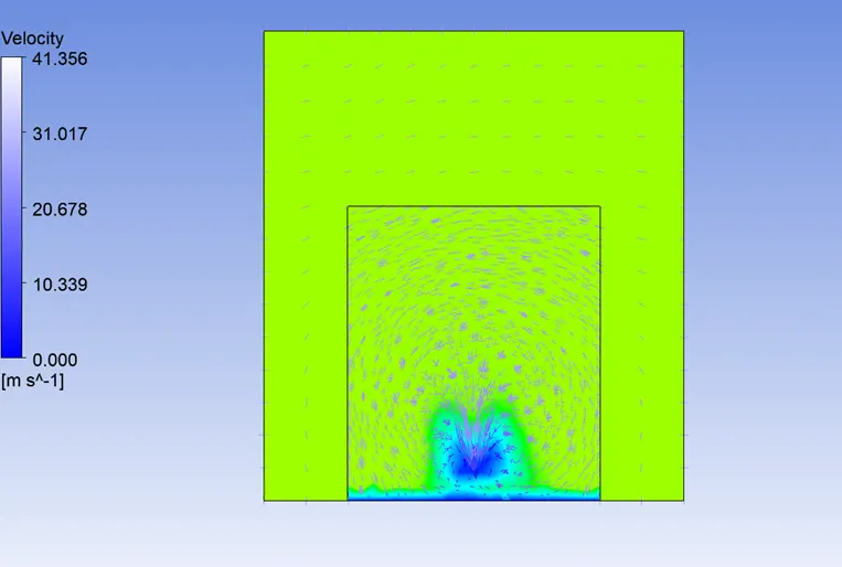
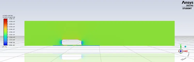
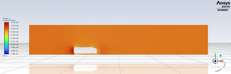
The findings from the countours in this case are not up to the necessary experimental values, thus further refinement is needed to get the results to the appropriate levels. Additionally, we can see from the velocity countour that low pressure is building because of the slant angle.

Significance of the point of separation –

The flow around the Ahmed body has several flow separations from the front to rear of the vehicle. The flow recirculation caused by this flow detachment contributes the vehicle’s drag. The location points at which the flow separates determines the size of the separation zone, and accordingly the drag force, thus an exact simulation of the wake flow and of the separation process is essential for the accurate result of drag predictions.

• Inner Enclosure -

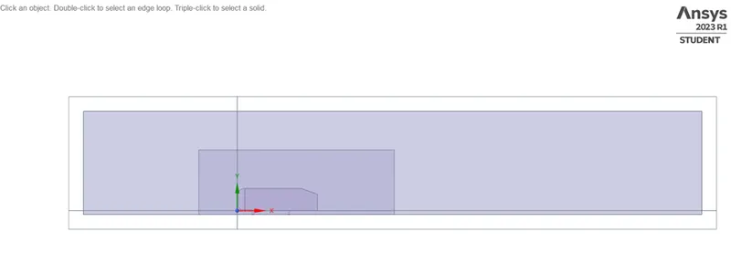
• Right face is located at a distance of 1 m from the right side face of Ahmed body along the X axis.
• Left face is located at a distance of 0.5 m from the left side face of Ahmed body along the X axis.
• Top face of the encloser is at a distance of 0.5m from the top side face of the Ahmed body along the Y axis.
• The bottom face of the encloser is attached to the bottom face of the Ahmed body along the YZ plane.
• The front and back face of the encloser is at a distance of 0.26 m along the Z axis.

• Meshing -

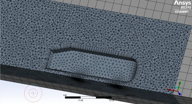
We can utilise various meshing processes for this model, assigning named selections for the inlet, outlet, symmetry wall, and car wall.

We adhere to three stages in this.

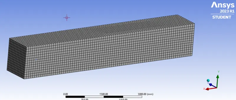
1. Meshing will be carried out for the outer enclosure using the Multizone approach, resulting in the creation of a Hexa mesh with an element size of 0.01 m.

2. To further enhance the inner enclosure, we use the body scaling method. The element size used for this is 0.05 m.

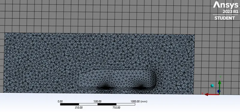
3. Then, we create the inflating layer, which aids in caputuring the flow in a much finer manner and ensures that the mesh is perfectly captured along the body. We assume there are 6 layers of inflation, making the total thickness 0.0036.

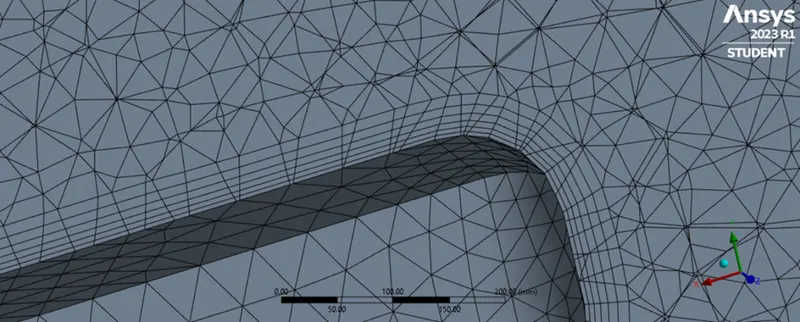
We use Y+ = 100 to calculate the total thickness.

The calculations required to arrive at these figures,

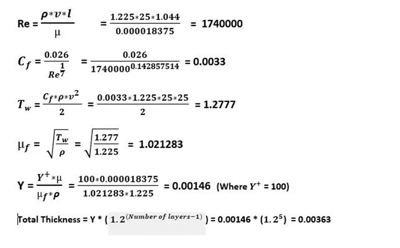
Where ,

ρ , µ are fluid density and viscosity ;

v is the free stream velocity ;

L is characteristic length ;

Uf is frictional velocity ;

Tw is wall stress ,

Cf is skin friction coefficient

Setup–

Solver type : Density based

Check the Energy equation

Turblent Model : K-Omega SST model

Fluid Material : Air

Boundary Conditions–

Inlet velocity : 25 m/s

Outlet pressure : 0 pa

Symmetry : For side walls

Wall : Bottom ,

Creating a surface plane to observe the contours.

Results-

1. Pressure & Velocity Contours

2. Scaled Residuals

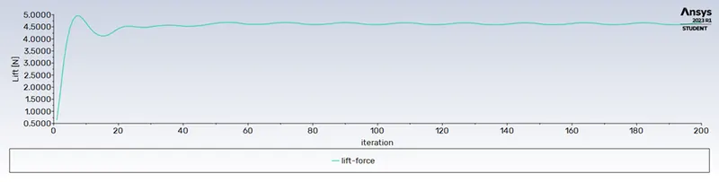
3. Drag

4. Lift

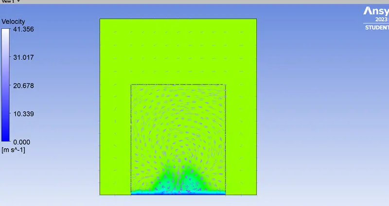
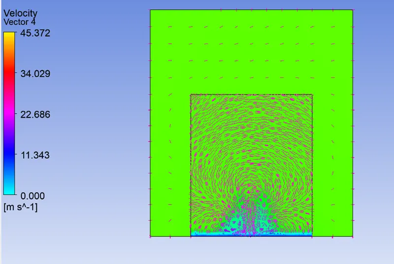
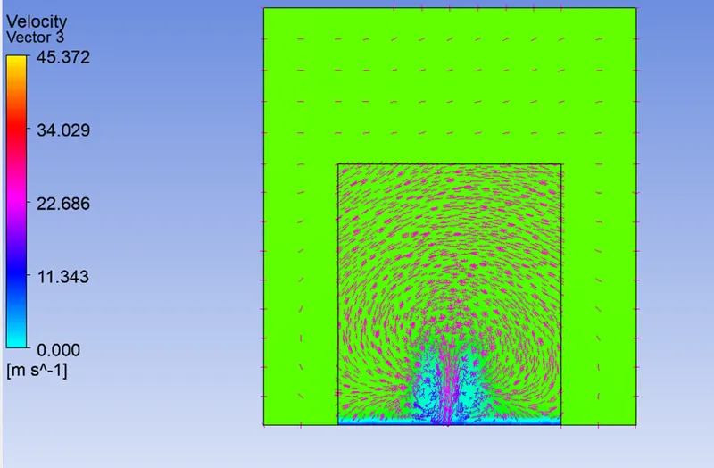
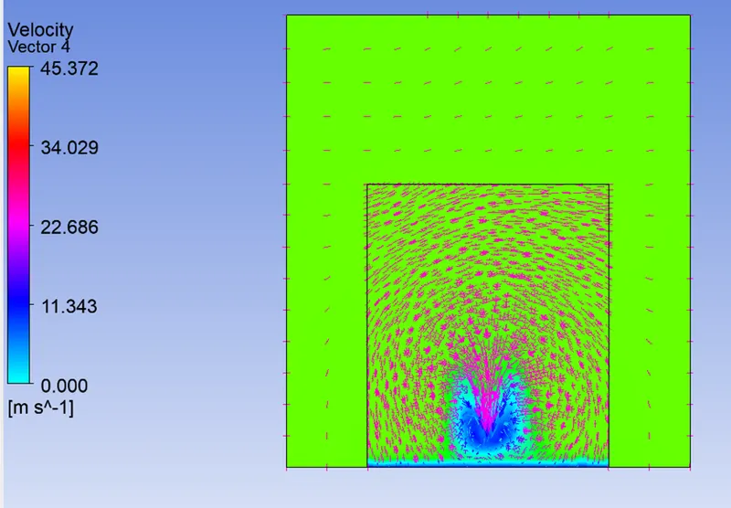
5. Velocity Conturs near wake region

Final Refinement –

To get more accurate results we are using more refined meshing for the geometry. The only change that we are going to do is we are reducing the element size of inner enclosure to 35mm.

Results -

1. Velocity & Pressure Contours

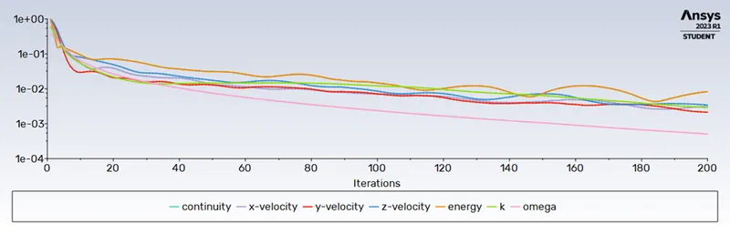
2. Scaled Residuals

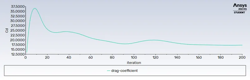
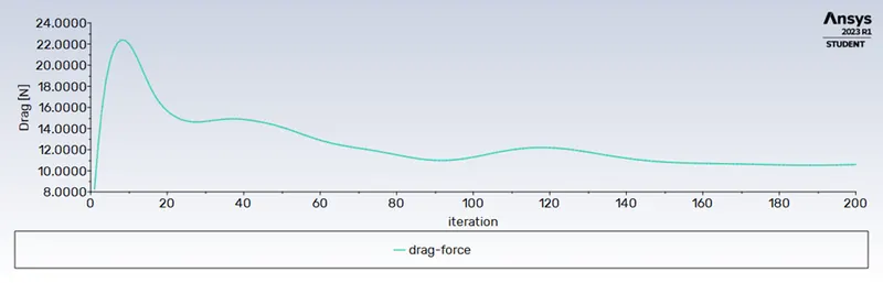
3. Drag

4. Lift

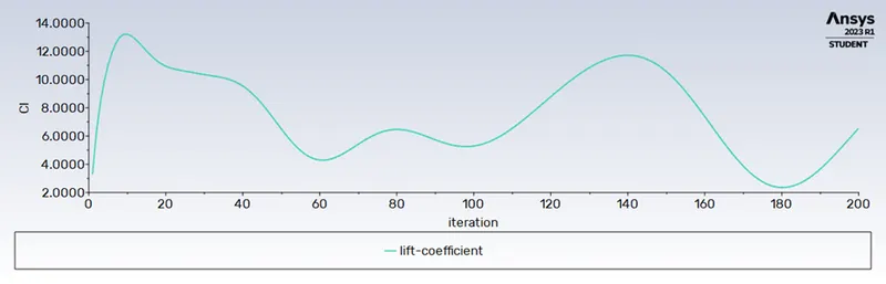
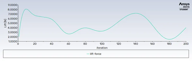
5. Velocity Contours near wake Region

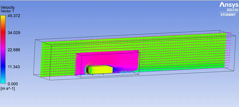
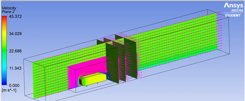
Comparison -

	Multi Zone	Body Zone	Total Thickness	Drag Coef.	Lift Coef.	Element Size	Drag Force	Lift Force
Baseline mesh	Baseline	-	-	0.75	0.64	500030	18.80N	6.91 N
Refined Mesh	100mm	50mm	3.63mm	0.29	0.012	142179	11.16 N	4.66 N
Final Refined Mesh	100mm	35mm	3.63mm	0.17	0.0978	329307	10.55 N	4.02 N

Conclusion –

1.The post-CFD results at the region of mesh overlapping were erroneous based on executing a baseline simulation.

2.Grid independency test results are most accurate when they are near to experimental data. The inaccuracy is greatly decreased by reducing the mesh size using the y+ factor.

3.The y+ is selected to provide an accurate estimate of the velocity and pressure contour plots.

4.As y+ is increased, the flow separation and appearance of vortices become more pronounced. As can be observed, baseline meshing does not correctly capture wake creation; however, after mesh refinement, the flow is properly caught.

Click here for Simulation Files