Steady-State Simulation on Mixing Tee

Aim-

To set up steady-state simulations to compare the mixing effectiveness when hot inlet temperature is 36^oC and the cold inlet is at 19^oC for the given geometries as per the problem statement given in the question.

Procedure-

1. Case 1
   • Short mixing tee with a hot inlet velocity of 3m/s.
   • Momentum ratio of 2, 4.
2. Case 2
   • Long mixing tee with a hot inlet velocity of 3m/s.
   • Momentum ratio of 2, 4.

1.Case 1 (A)

• Short mixing tee with a hot inlet velocity of 3m/s.
• Momentum ratio of 4.
• Viscous model K-epsilon

To initiate the simulation process in ANSYS we have to drag and drop the Fluid Flow(Fluent) Option in to the workplace. Following is the sequence and series of operations/steps for the simulation in ANSYS

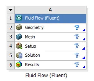
To load the geometry part and to setup we have to select “Geometry” option. Which will start SpaceClaim Application. By which we can prepare the geometry. After opening the application we have to open the CAD file.

As for the particular CFD application we are interested in the volume where the fluids interact. To extract the volume SpaceClaim provides a function in prepare tab called “Volume Extract”. After clicking on the on the Volume Extract we have to select the edges of the required volume and then click on green mark which will complete the extraction process and create a new special volume. Also we have to hide and use supress for physics option to exclude the unwanted surfaces in further calculations.

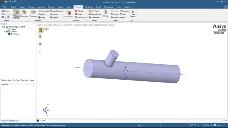
After geometry preparations we move to the Meshing stage.

To add the appropriate meshing we have to name the particular boundaries. To create named selections we have to right click on particular face and select “Create Named Selection”.

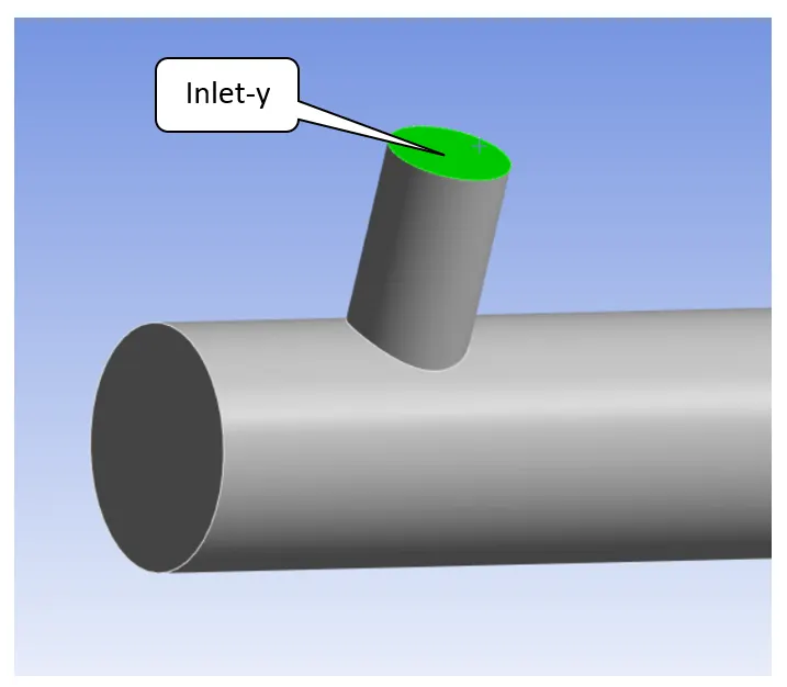
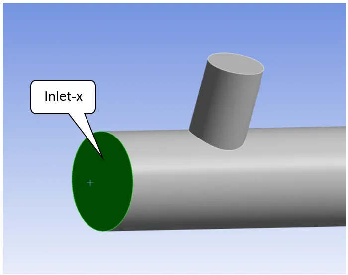
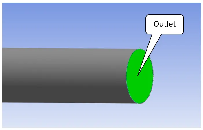
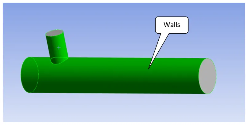
After this naming process, we are ready to give meshing. As this is introductory CFD meshing we are leaving sizing parameters as it is. And generate the mesh.

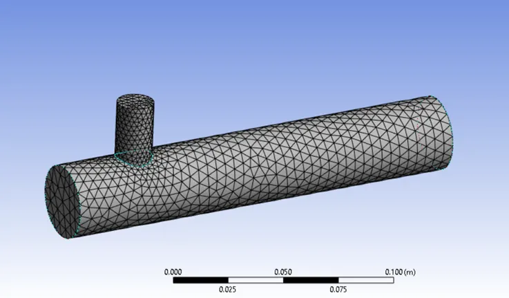
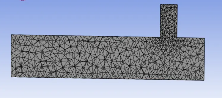
To check whether we can run the simulation successfully or not we have to check the element quality. We need to ensure that the minimum element quality is above 5%. In this case it is 30%

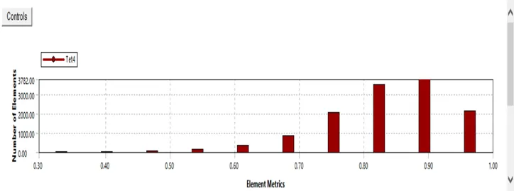
This completes our 2^nd step. Now the next step is “SETUP”

After selecting Setup option, we choose parallel processing with 4 cores option and double precision option. After opening the Fluent GUI our first task is to check the mesh quality. Click on Check and we are ready to go.

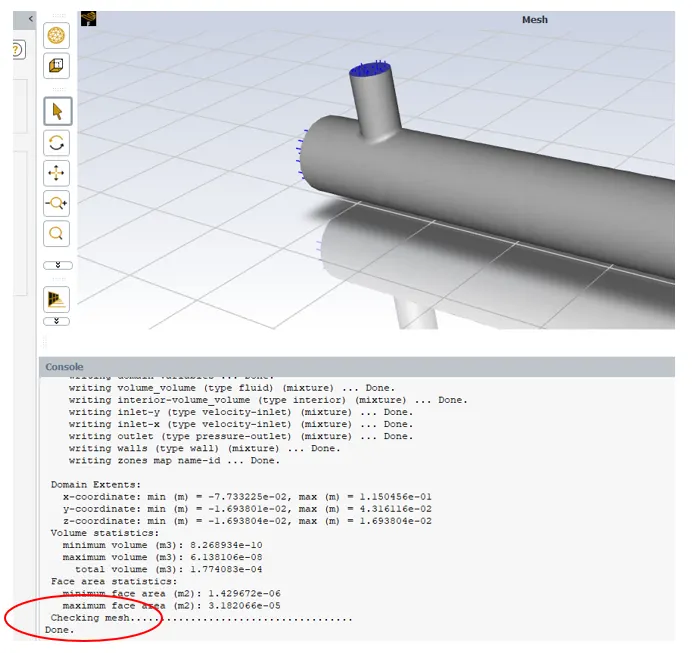
The next step is to setting up the physics in Fluent.

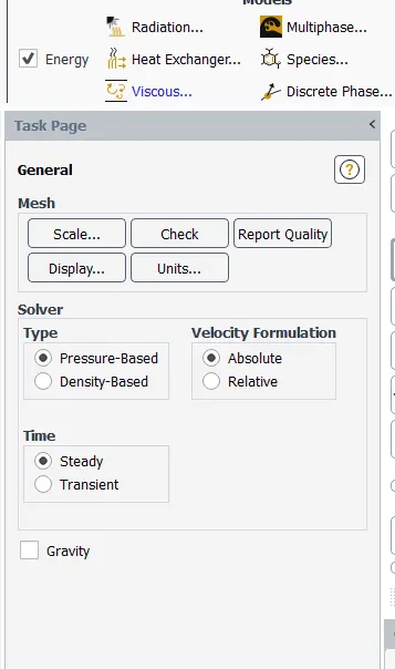
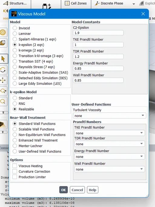
As we are using K-epsilon viscous model

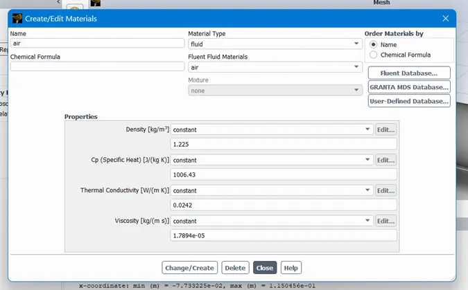
Then Material selection,

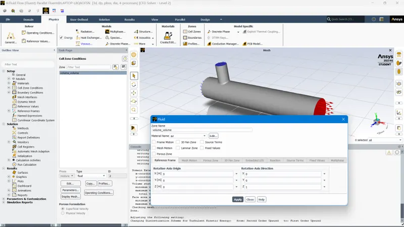
Then we need to assign boundary conditions. For that we have to select first Cell Zones option in Zones. Then we have to assign volume region i.e. our meshed region.

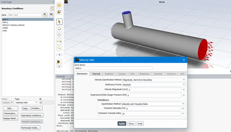
Next parameter is boundary,

Name of Boundary	Velocity Magnitude(m/s)	Temperature(deg. Celsius)
Inlet-x	3	36
Inlet-y	12	19

To monitor temperature at the outlet we need to define area-weighted average from definitions tab,

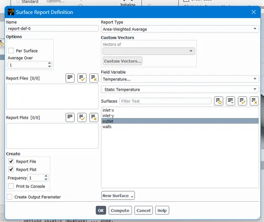
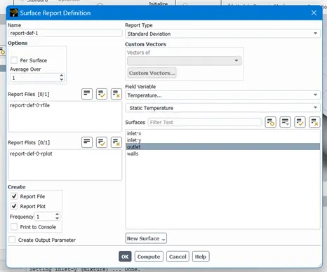
Now, in order to understand the effectiveness of mixing we are defining the standard deviation parameter in definitions,

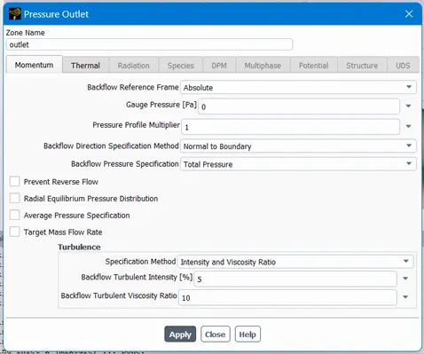
Also we have checked the pressure at outlet in boundary condition is zero,

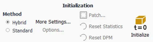
For solving we initialize from solution tab,

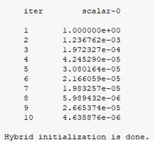
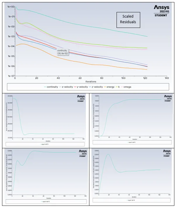
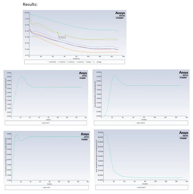
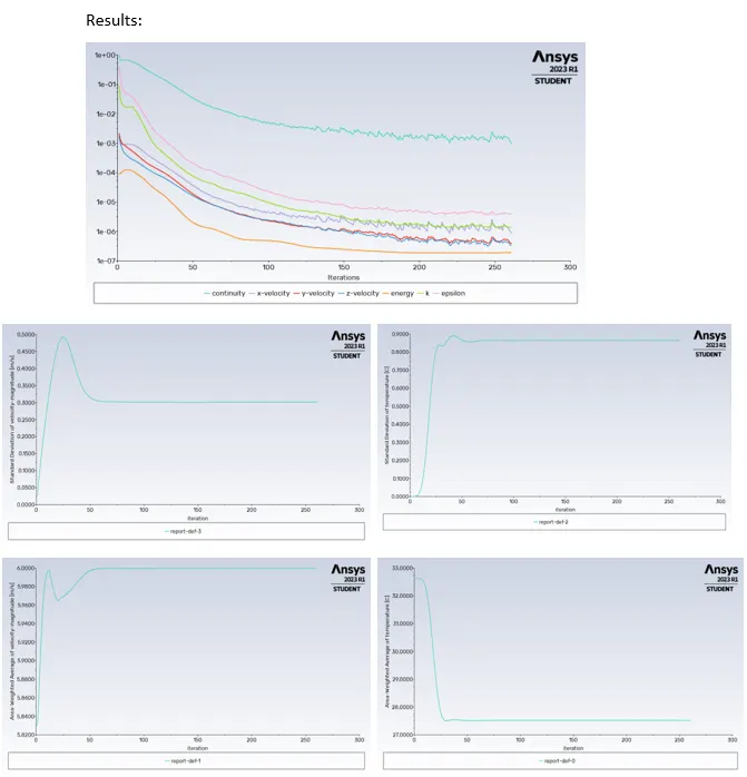
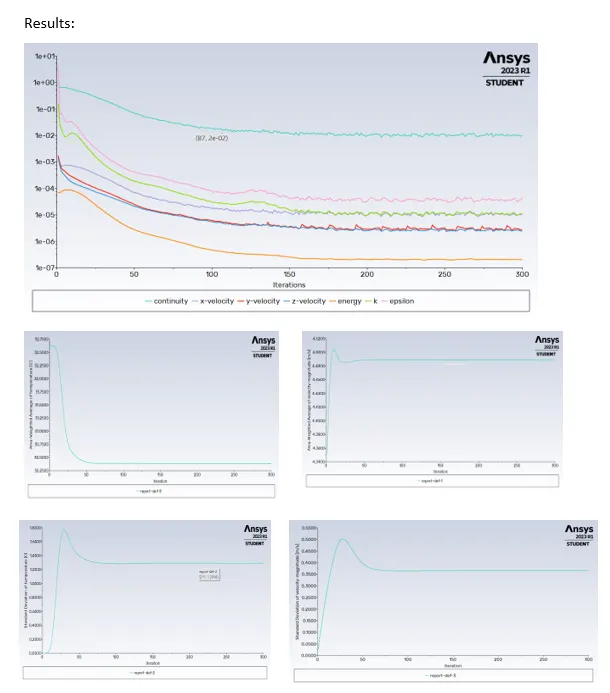
Now we are ready to run the solver. We are solving for 300 Iterations and here are the results of different reports and residuals,

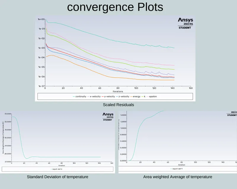
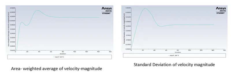
Now, the next stage is to post process this solved simulations this can be enabled by double clicking on results in workbench.

To see the velocity and temperature distribution we need to insert plane in the geometry.

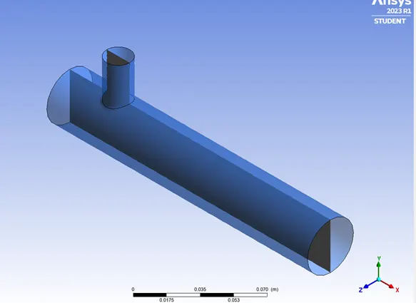
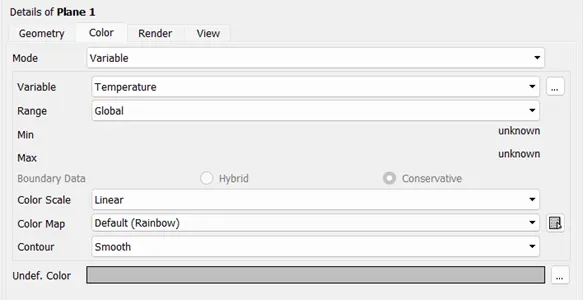
And apply variable colour to the plane with temperature distribution.

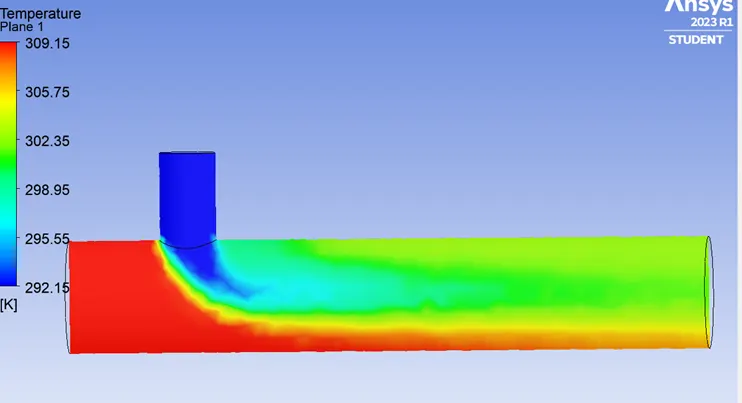
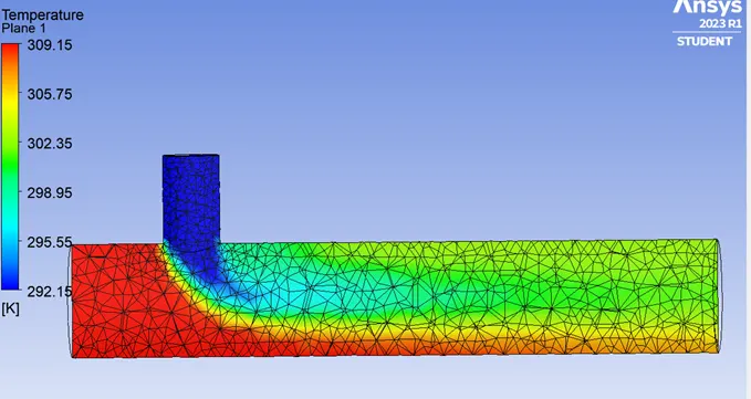
To generate more defined mesh we changing mesh size to 3e-3.

After updating and resolving we can see that the results are now more refined.

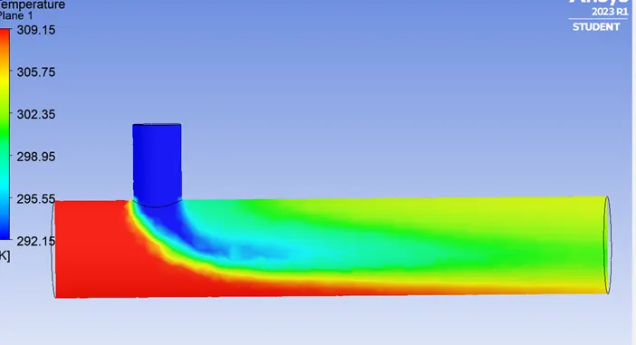
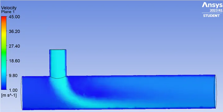
2.Case 1 (A)

• Short mixing tee with a hot inlet velocity of 3m/s.
• Momentum ratio of 4.
• Viscous model K-omega

Convergence Plots

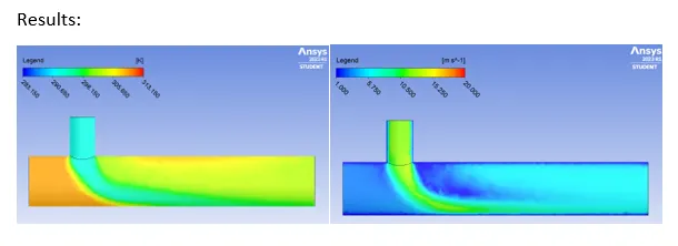
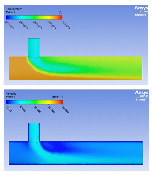
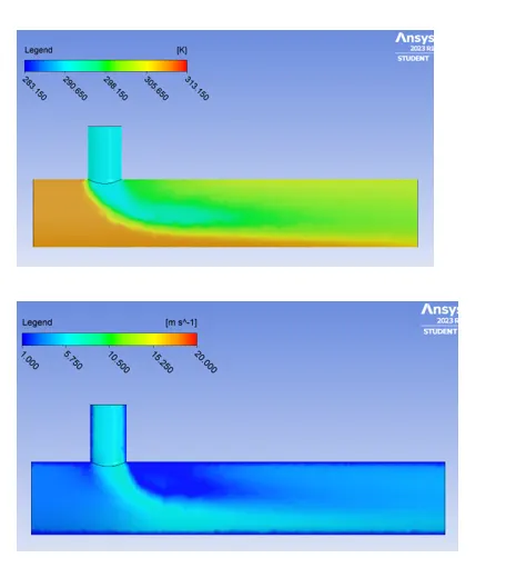
We can notice the flow difference between k-epsilon Realizable and k-omega SST in the contour graphic above. Let's first examine what makes them distinct.

Image of results comparing

K-Epsilon

The K-epsilon turbulence model is the most popular model used in CFD to calculate mean flow characteristics under turbulent flow conditions, as we observed in our first simulation. It is a two-equation model that uses two transport equations to describe turbulence (PDEs). The rate of dissipation of turbulent kinetic energy (k) is the second transferred variable after turbulent kinetic energy (k), which are the first two carried variables.

The mechanism that impacts the turbulent kinetic energy is the main topic of k-epsilon.

That's the reason we are using K-epsilon model for further cases

K-Omega

Several aerodynamic applications use the SST k-omega turbulence model, which is a two-equation eddy-viscosity model. It is a hybrid model that combines the k-epsilon and k-omega Wilcox models. The Wilcox model close to the wall and the k-epsilon model in the free stream are both activated by the blending function F1. This guarantees that the proper model is applied via the flow field.

Main Difference

The viscous sub-layer flow may be accurately simulated using the k- omega model. The k-epsilon model, however, is superior for predicting flow in areas far from the wall.

Compared to many other turbulence models, the SST model is less sensitive to free stream circumstances (Flow outside the boundary layer).

The k-omega model is assisted by the shear stress limiter in preventing an accumulation of excessive turbulent kinetic energy close to stagnation spots.

If we look at our simulation graphic, we can see that the k-omega model's flow is more laminar and does not produce suitable turbulent outcomes, whereas the k-epsilon model's simulation produces proper mixing of the two air streams.

Since there are no barriers in this particular situation, we will use the k-epsilon approach for subsequent simulations.

3.Case 1 (B) MR2

• Short mixing tee with a hot inlet velocity of 3m/s.
• Momentum ratio of 2.
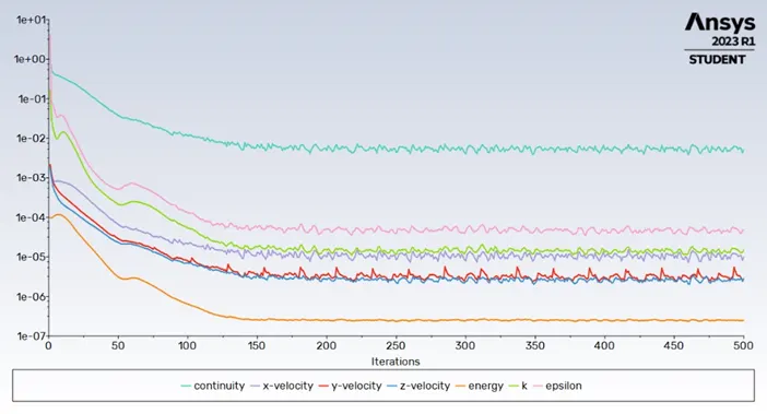
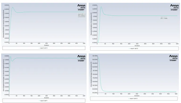
• Viscous model K-epsilon

4.Case 1 (B) MR2

• Short mixing tee with a hot inlet velocity of 3m/s.
• Momentum ratio of 2.
• Viscous model K-omega

5.Case 2 (A) MR2

• Long mixing tee with a hot inlet velocity of 3m/s.
• Momentum ratio of 4.
• Viscous model K-epsilon

By using the above procedure we can also calculate this case,

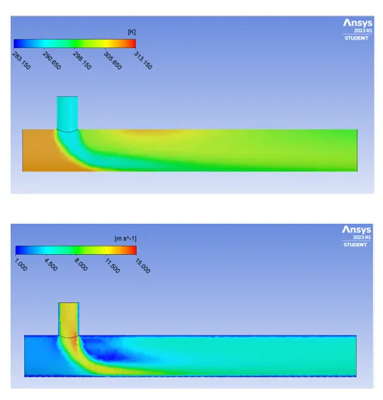
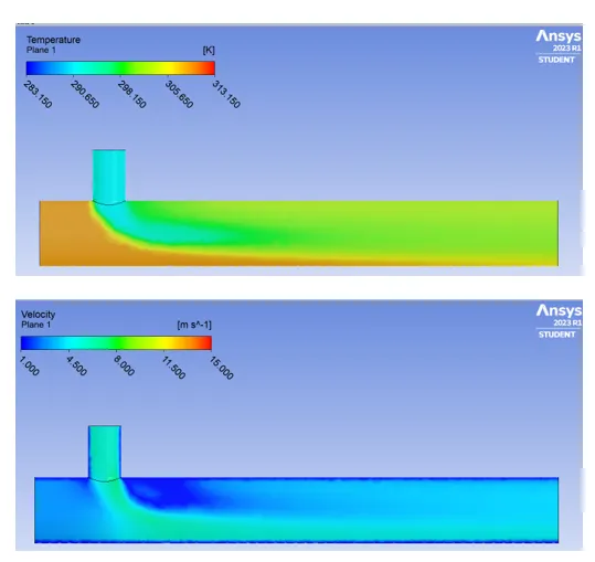
6.Case 2 (B) MR2

• Long mixing tee with a hot inlet velocity of 3m/s.
• Momentum ratio of 2.
• Viscous model K-epsilon

Conclusion:

1.The k-omega model predicts flow close to the wall, while k-epsilon models suggest flow virtually far from the boundary (wall). The k-epsilon approach is utilised because in this situation we require a flow simulation turbulence model far from the wall.

2.The convergence time grows along with the element count. So, after successfully collecting the rough findings from the coarse mesh simulation, we may enhance the mesh quality and achieve the final exact results. Doing so saves a significant amount of time and is also very beneficial for the mesh independence test.

3. High flow velocity can improve mixing at the exit quite well. As a result, a larger momentum ratio results in improved fluid stream mixing at the outflow.

4. Diffusion flow always results in slightly better mixing of two fluids, hence the length of the mixing tee grows.

5. Last but not least, in the aforementioned situations, it is crucial to utilise a short mixing tee with a momentum ratio of 4, but one must also take into account the diffusion of flow throughout the length of the mixing tee; in this instance, a long mixing tee with momentum will be a better choice.

https://drive.google.com/file/d/15NySWdLkNgwIZ7Mfaf2PFOoAwlHwwnII/view?usp=sharing