CHT Analysis on Exhaust port

Aim – To Perform Conjugate Heat transfer (CHT) Simulation on Exhaust ports.

Introduction –

• Conjugate Heat Transfer (CHT) analysis –

By transferring thermal energy at their interfaces and transporting it by conduction within solids and furthermore via convection within fluid domains, conjugate heat transfer analysis enables the simulation of heat transfer between solid and fluid domains.

By simultaneously resolving all relevant solid and flow field heat transfer processes, conjugate heat transfer analysis may accurately forecast heat transfer.

The combination of heat transmission in fluids and heat transfer in solids is known as conjugate heat transfer.

Convection typically dominates in fluids while conduction frequently does so in solids. Conjugate heat transfer is seen in a variety of circumstances, including thermal radiation, free and forced convection in gases and fluids, and conduction in solids.

• Need of CHT analysis –

By simultaneously resolving all the relevant solid and flow field heat transfer processes, such as conduction through solids, free and forced convection in the gases/fluids, and thermal radiation, conjugate heat transfer (CHT) analysis can effectively estimate heat transfer.

As wall heat transfer coefficients and their local changes on surfaces are directly estimated within the model rather than relying on reduced empirical estimates, the CHT approach has an advantage over FE thermal evaluations. Hence, the CHT technique provides advantages for applications where heat transmission is either non-uniform or challenging to estimate empirically.

• Applications of CHT analysis –

1. After-Treatment

In Urea/SCR aftertreatment systems, predicting and reducing the production of urea deposits is a significant difficulty. Spraying urea-water solution into the engine exhaust system causes a liquid layer to impinge on the wall. The heat transfer between the film and the wall is crucial to record because it affects the decomposition of urea and the production of unwanted deposits. You can find the places that are susceptible to wall deposition by predicting the temperature of the wall.

2. Electromobility

Several E-mobility system components require effective cooling solutions. Electric motors produce a lot of heat because of their high-power densities. High temperatures in a motor can led to the demagnetization of the permanent magnets and the failure of the winding insulation if it is not appropriately cooled.

3. Pumps & Compressors

The precision of the simulation is increased, and usable temperature information is produced by resolving the spatially variable surface temperature distributions in pumps and compressors. Thermal expansion, for instance, has an impact on the space between the rotors of a twin screw compressor. If that effect is not considered, the simulations will anticipate leakage flows incorrectly and your results will be less accurate.

4. Internal Combustion Engines

The internal combustion engine industry is moving away from modelling individual components and towards simulating the overall system. The temperature boundary conditions inside the cylinder determine how accurately the projected combustion will occur. By taking into account heat transmission in the metal parts (such as the cylinder head, liner, piston, etc.), the cylinder wall's temperature is now anticipated as part of the complete-system simulation rather than being determined by the user. By lowering the dependency on assumed boundary conditions, this increases the predictiveness of the total simulation results.

• Heat Transfer Coefficient –

The heat transfer coefficient or film coefficient, or film effectiveness, in thermodynamics and in mechanics is the proportionality constant between the heat flux and the thermodynamic driving force for the flow of heat (i.e., the temperature difference, ΔT)

The overall heat transfer rate for combined modes is usually expressed in terms of an overall conductance or heat transfer coefficient, U. In that case, the heat transfer rate is

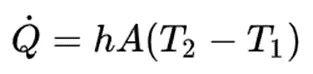
Where,

A, is the surface area where the heat transfer takes place, m2

T_2, temperature of the surrounding fluid, K

T₁,temperature of the solid surface, K

The general definition of the heat transfer coefficient is,

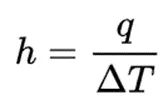
Where,

q, heat flux, W/m2; i.e., thermal power per unit area, q = dQ'/dA

h, heat transfer coefficient, W/(m2•K)

ΔT, difference in temperature between the solid surface and surrounding fluid area, K

It is used in calculating the heat transfer, typically by convection or phase transition between a fluid and a solid. The heat transfer coefficient has SI units in watts per squared meter kelvin: W/(m2K).

The heat transfer coefficient is the reciprocal of thermal insurance. This is used for building materials (R-value) and for clothing insulation.

Geometry Setup –

• In the first step we have to import the geometry in SpaceClaim for further processing.

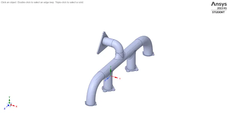
• To repair extra surfaces present in the geometry we have to enable Extra Edges and remove the extra surfaces.
• After this we have to extract the volume by using volume extract command.

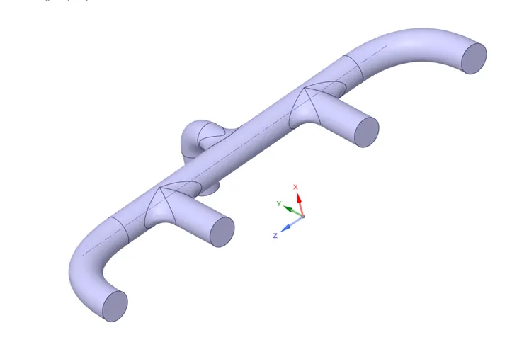
• Then rename the volumes created i.e.., Solid-volume and fluid-volume with this our geometry setup is complete.

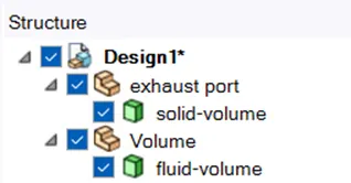
After this, we generate the mesh by taking all the default values. The mesh is generated fine but if you zoom it you can observe there is no connection between the inner volume and outer volume.

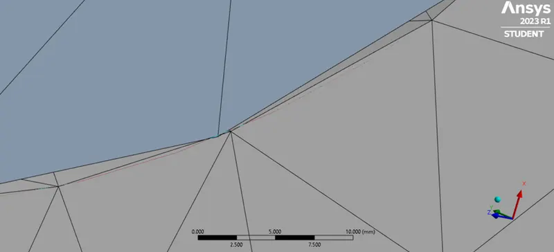
This problem can be solved by using share topology and at last share prep under the workbench tool must be selected to achieve conjugate heat transfer between the fluid and wall. This will ensure that the heat transfer is recorded from intake to outlet of the wall.

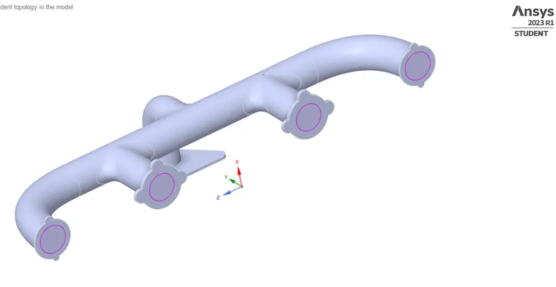
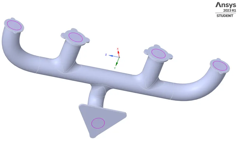
Meshing –

1. Create named sections

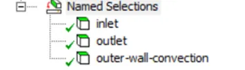
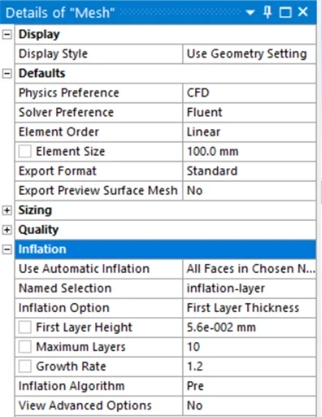
1. Go for default baseline mesh setup. i.e.., Element size of 150 mm.

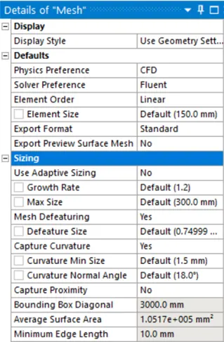
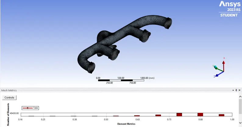
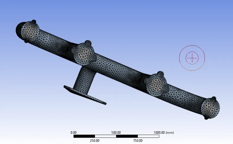
3. Inflation Layer

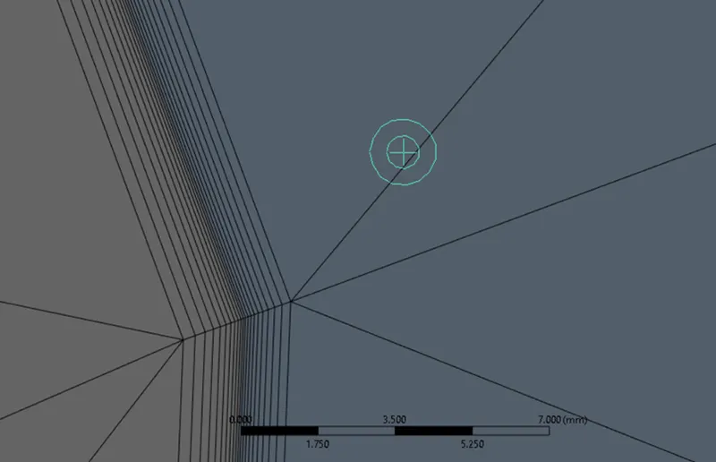
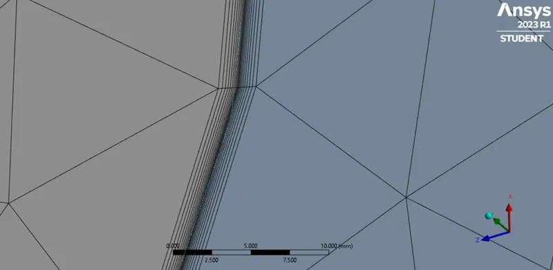
• Due to the importance of the interface, where we wish to calculate the heat transfer, we must use that area and make inflated layers in order to precisely record the flow and calculate the data.
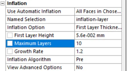
• In the global mesh, choose the inflation option. To use automatic inflation, select all faces in the selected named selection, and to utilise the inflation layer we just specified, select named selection.
• Additionally, we provide first layer thickness for the inflation option based on the y+ value and the turbulence model we employ.Because of the k-omega SST turbulence model that we are using, y+ should fall between 0.1 and 5.Let's determine the thickness of the first layer.

1. U∞ = freestream velocity = 5 m/s
2. ρ = freestream density= 1.225 kg/m3
3. μ = dynamic viscosity= 0.000017894 kg/m s
4. L =diameter of the inlet(m) = 0.1662206 m
5. desired y+ = 1

=> Then Reynolds number, Re = (ρ*U∞*L)/μ = (1.225*5*0.1662206)/ 0.000017894 =56896.2319

=> skin friction coefficient, C_f = (0.026)/Re ^1/7 = 0.026/(56896.2319)^1/7 = 0.00544096214

=> wall shear stress, Tau_wall = (C_f*ρ*U∞^2)/2 = (0.00544096214*1.225*(5)^2)/2 =0.08331473276

=>friction velocity , U_friction = (Tau_wall/ρ)^1/2 = (0.08331473276/1.225)^1/2 = 0.26079115541

=> Therefore, first layer thickness , Δs = (y+ * μ)/(U_friction*ρ)=(1*0.000017894)/(0.26079115541*1.225) = 0.0000560116653 m = 0.0560116653 mm

• Now that we have the first layer's thickness, let's give it together with a maximum of 10 growth layers and an inflation layer growth ratio of 1.2.

4. Mesh Sizing

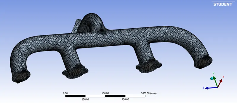
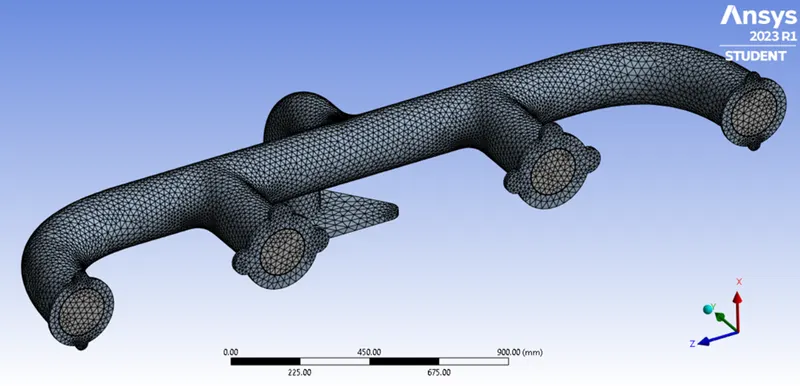
By utilising sizing, we are finely meshing the internal fluid domain. To do this, right-click on the mesh and select "sizing." Geometry: We choose the inner fluid volume by hiding the exterior component and providing a size of 50 mm. The inner fluid volume will be refined more finely when you generate the mesh once again.

Fluent Setup –

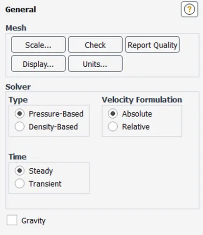
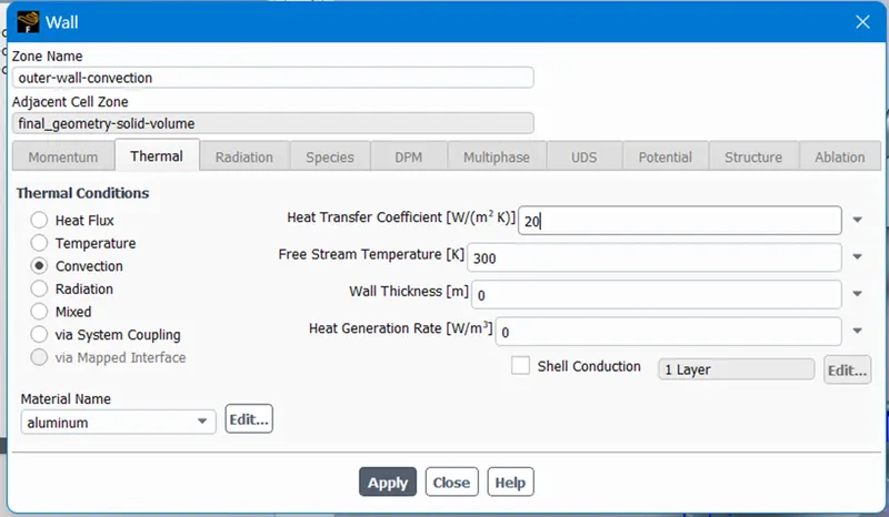
• Choose a pressure-based solver applying the steady-state time simulation and absolute velocity formulation under the general settings after updating the mesh open fluent setup.
• Select the energy option under physics since we are dealing with temperature attributes.
• Enter the boundary values at the inlet with a velocity of 5 m/s and a temperature of 700 k. Convection type should be selected for the outer wall convection boundary, and the heat transfer coefficient should be entered as 20.
• Properties choose aluminium as the solid material and air as the fluid material under "Materials."
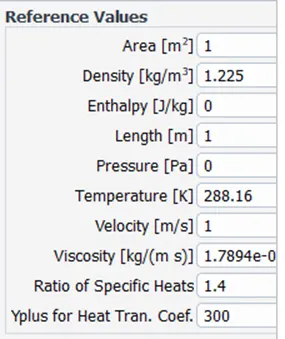
• In accordance with the geometry and inlet boundary conditions, enter the reference values.
• In order to acquire a convergent solution, initialise using the hybrid initialization and simulate for 250 iterations.

Results –

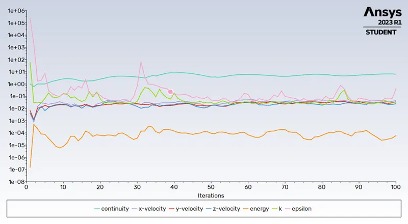
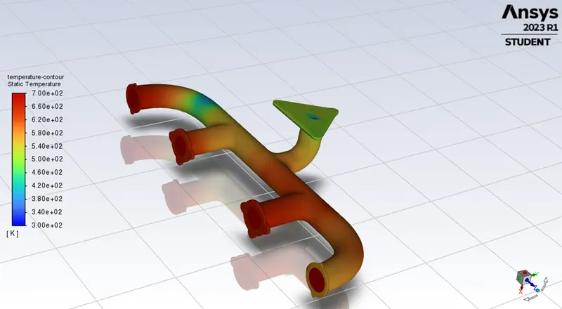
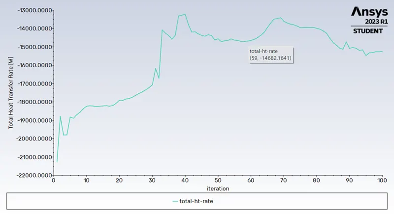
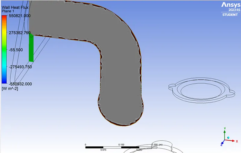
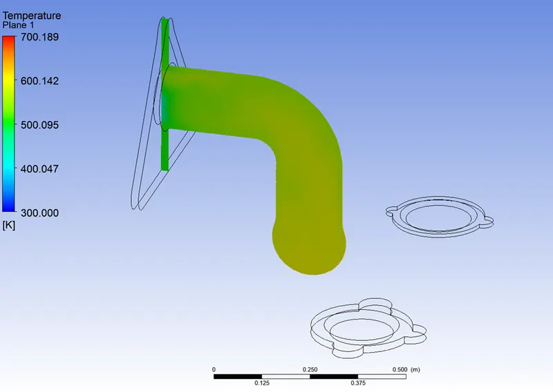
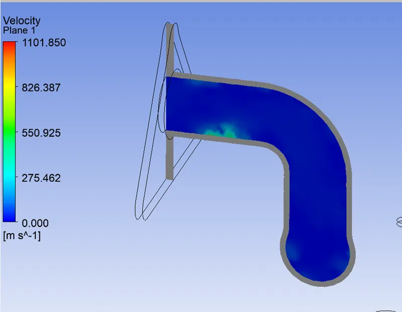
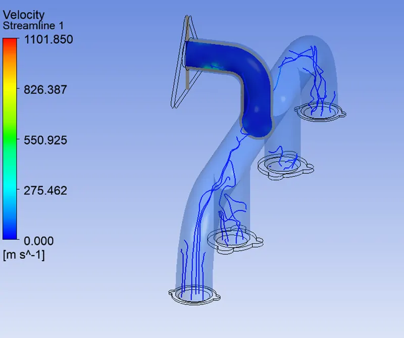
As we are observing this the K-Epsilon Model is not calculating properly we are going with K-Omega model.

Case 2 Refined mesh -

element size =100mm

sizing element size=20mm

no. of elements= 510754

viscous model=k-omega

inlet velocity =5m/s

inlet temperature=700k

HT co-efficient=20W/m^2-k

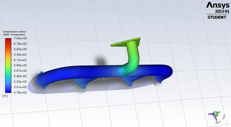
Results -

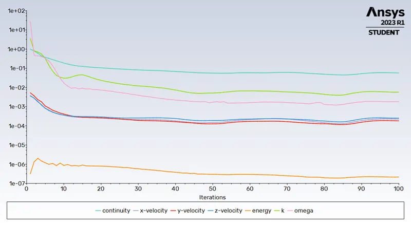
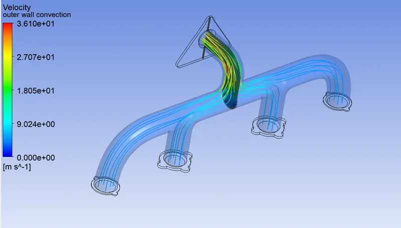
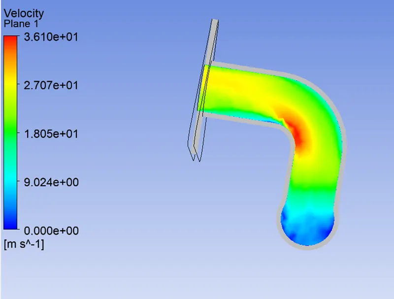
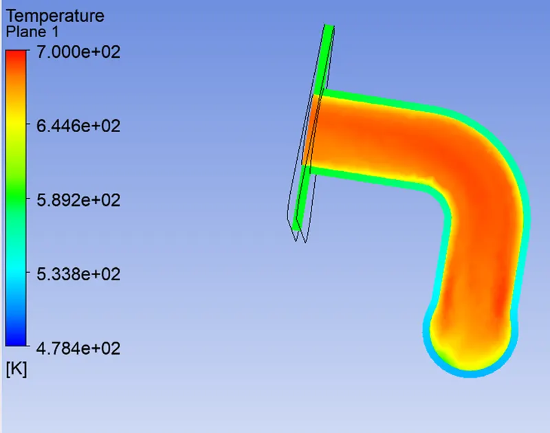
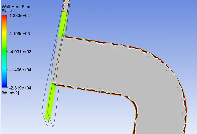
Conclusion -

Cases	Viscous Model	No. of Elements	H.T Rate (W)	Wall H.T. Flux (W/m2)
1	K-Epsilon	369710	-15245.8	550821
2	K-Omega	510754	-10914.6	13328

Since we are dealing with temperature, we can increase accuracy by comparing 2 examples using the k omega model.

In the k-omega model, the wall heat co-efficient is higher than in the k epsilon model.

In all circumstances, there is no change in temperature.

Y plus needs to be computed based on the solvers.

How would you confirm the accuracy of the HTC projections based on the simulations? What elements influence the prediction's accuracy?

Answer to this question is that,

According to Bernoulli's mass conservation principle mass is conserved in our model which is clearly explained below.

Let us assume the flow rate from each inlet as Q1, Q2, Q3, Q4 respectively, and Q5 be the flow rate(outflow) from the exhaust manifold.

As mass is neither created nor destroyed, mass flow rates are also balanced as below,

Q1+Q2+Q3+Q4=Q5Q1+Q2+Q3+Q4=Q5 -------(1)

we have Q=ρ.A.VQ=ρ.A.V -------(2)

now the equation 1 becomes

A1.V1+A2.V2+A3.V3+A4.V4==A5.V5

as it is an incompressible flow to compensate for the mass flow, velocity is increased, and the overall mass flow rate is conserved.

As velocities are high, the Reynolds number at the outlet manifold will be high.

Nu=f(Re, pr) for forced convection applications,

Nu=hD/k

from the above equations

Nu∝Re,

Nu∝h,

hence, Re∝h

Our calculations revealed that the bend section of the outlet manifold has high velocities, leading to increased Reynolds numbers and high heat transfer coefficients.

As a result, forecasts based on our simulations can be regarded as accurate.

Factors that affect prediction accuracy include:

• As seen in the contours above and the maximum values of relevant parameters like velocity and heat transfer coefficient, mesh quality has a significant impact on the accuracy of the anticipated value from our simulations.
• In our example, HTC, a proper y+ value aids in the calculation of the entire layer thickness from the wall for better recording of impacts near walls.
• It is crucial to employ an appropriate turbulence model in accordance with the y+ value.
• One of the most crucial elements that guide all computations in solving equations is the use of appropriate solvers.
• Layers of inflation and boundary circumstances

Click Here to Download Ansys Files