Week 9 - FVM Literature Review
In CFD, the three mainly used numerical method based solvers to solve the governing equation (i.e Navier Stoke's Equation), are Finite Volume Method (FVM), Finite Difference Method (FDM) and Finite Element Method (FEM).
Finite Volume Method
It is a discretization technique for partial differential equations, especially those that arise from physical conservation laws. FVM uses a volume integral formulation of the problem with a finite partitioning set of volumes to discretize the equations. FVM is in common use for discretizing computational fluid dynamics equations. The Finite Volume Method determines the property over a control volume and assumes that it is concentrated in its geometric centre.FVM is widely used as it can be applied for complex geometries and moving parts.
Finite Difference Method
The Finite difference method determines the property at a single node/point. This is the oldest method of all three, but this is obsolete. It uses a topologically square network of lines to construct the discretization of PDE. FDM converts a linear ordinary differential equation (ODE) or non-linear differential partial equations into a system of equations that can be solved by matrix algebra techniques.
Interpolation Scheme
The approximations of surface and volume integrals require values of the variable at locations other than the computational nodes of the control volume. Values at these locations are obtained using interpolation formulae.
Methods of Interpolation
Upwind Interpolation
Linear Interpolation
Quadratic Upwind Interpolation
Hybrid, TVD and ENO interpolation schemes.
As an example, lets consider a simple case of steady-state one-dimensional convection and diffusion
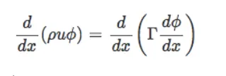
where ϕ is our scalar solution variable
ρ is the density
u is the velocity
T is the diffusion coefficeint
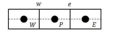
The above picture represents three neighbouring control volumes, which we are going to use for deriving the discretiztion equation.
Integration of the governing differential equation over the control volume around grid point P yields.

Evaluation of LHS of the above equation requires values of ϕ over faces e and w . These values are calculated by employing the above-given interpolation schemes.
a) Upwind Interpolation Scheme
This scheme takes into account the direction of fluid flow and based on it the value of the solution variable at the face is approximated by its value at the upstream computational node. For example, if the fluid is moving from west to east, then

and if the fluid is moving from east to the west, then

b) Linear Interpolation Scheme
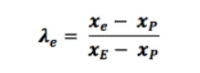
In order to approximate the value of a variable at the control volume face centre by two nearest computational nodes location e . This is equal to a central difference scheme of the first-order derivatives. It is second-order accurate and produce oscillatory solutions. The relation for linear interpolation is given below.
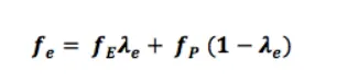
where
Flux Limiters
When computing the variable gradients, they tend to toggle and are not bound to a particular value and keep jumping. This occurs due to discontinuity, having a flux limiter will help to bound the gradient value and giving a stable solution
For convective fluid flow, it is seen that low order schemes are usually stable but quite dissipative in nature around the points of discontinuity or shocks while the higher-order schemes are unstable in nature and shows oscillations in the vicinity of discontinuity or shocks. Highly accurate and oscillation free schemes are known as high resolution schemes.
In order to make the scheme Total Variation Diminishing scheme (TVD), we must constrain or limit the range of of possible values of the additional convective flux
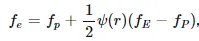 , which was originally introduced to make the scheme higher-order. Hence, the function ψ(r) is called a flux limiter function.
Flux limiter functions are used to fine-tune the higher order and lower order schemes in such a way that the resulting schemes gives a higher-order accuracy in the smooth region of the flow and maintains first order accuracy in the vicinity of shocks and discontinuities. For such a scheme TVD Scheme is employed.


where
 is Low precision flux (First order)
 is high precision flux ( higher order)
Conclusion
The finite Volume Method is really a powerful approach to solve the CFD problems. With the help of proper interpolation schemes and the accurate use of flux limiters in case of any discontinuities present, we can solve a wide range of CFD problems.