Week 8 - Simulating Cyclone separator with Discrete Phase Modelling

Challenge 8 – Simulating Cyclone Separator using Discrete Phase Modelling

Aim – To simulate the CFD of a cyclone separator and calculate the separation efficiency by varying the fluid inlet velocity, particle inlet velocity and diameter of particles

Introduction to the Cyclone Separator and several empirical models used to calculate the collection efficiency –

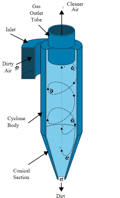
Working of a cyclone separator - A cyclone is a centrifugal separator in which particles, due to their mass, are pushed to the outer edges as a result of centrifugal force. Incoming air is automatically forced to adopt a fast-revolving spiral movement - the so-called “double vortex”. This double spiral movement consists of an outer stream, which flows downwards in a spiral, and an inner stream, which flows upwards in a spiral. At the interchange between both streams, air passes from one stream to the other. The particles which are present in the air are forced to the outer edges and leave the separator via a collection device fitted to the bottom of the separator.

4 empirical models to calculate the collection efficiency of a cyclone separator –

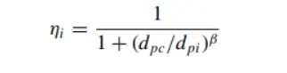
1. Lapple Model – It was created based on the force balance without considering the flow resistance. He assumed that any particle entering the cyclone is uniformly distributed across the inlet opening. The collection efficiency according to him was given by

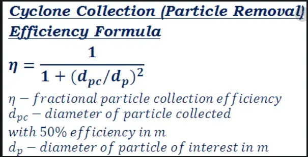
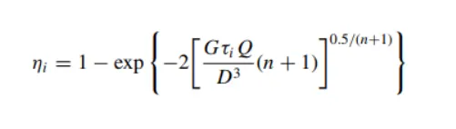
2. Koch and Licht Model – IN this particular case, this theory recognised the inherently turbulent nature of cyclones and the distribution of gas residence within the cyclone

The following assumptions were made

• The tangential velocity of a particle is equal to the tangential velocity of the gas flow
• The tangential velocity is related to the radius of cyclone by u Rn constant

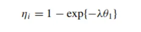
3. Li wang model – The li and wang model include particle bounce or re entrainment and turbulent diffusion at the cyclone wall. A two-dimensional analytical expression of particle distribution in the cyclone is obtained. The resultant expression of the collection efficiency is given by

4. Lozia and Leith model – this model is based on force balance. The model assumes that a particle is carried by the vortex endures the influence of two forces – a centrifugal and flow resistance. The collection efficiency can be calculated as -

Solving and Modelling Approach –

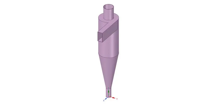
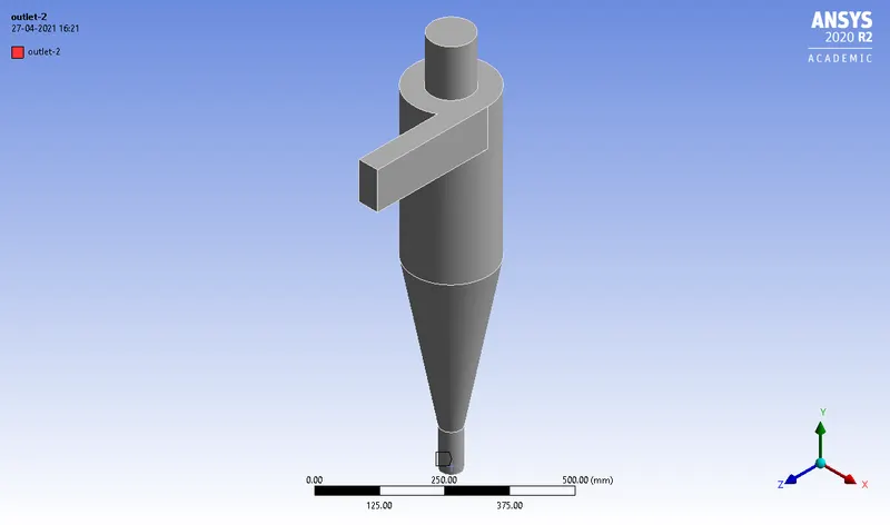
1. First and foremost, the step file of the cyclone separator was imported into Spaceclaim.
2. The prepare option was chosen and using edge select, the fluid volume was extracted by selecting the inner edges of inlet, outlet-top, and outlet-bottom.
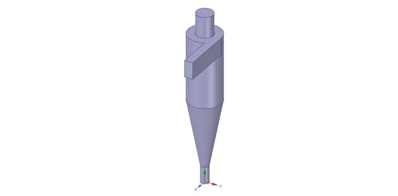
3. After obtaining the fluid volume, the remaining geometry was suppressed for physics, since the fluid will not be present in this region.
4. Finally, the fluid volume was further proceeded for meshing.

Meshing –

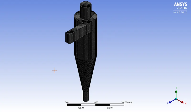
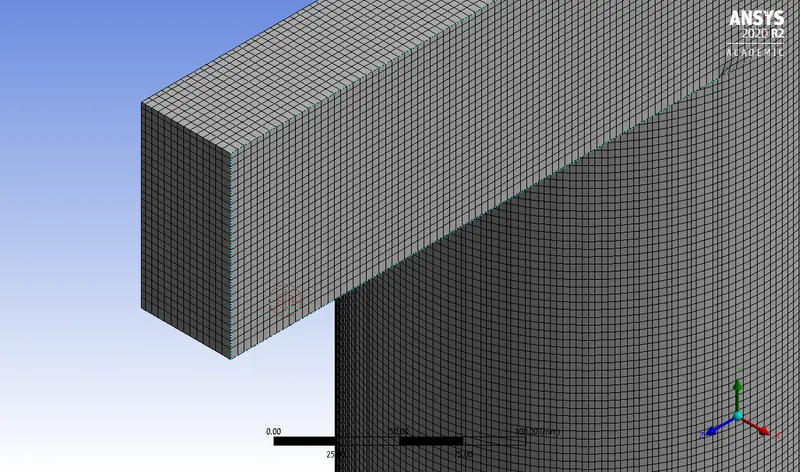
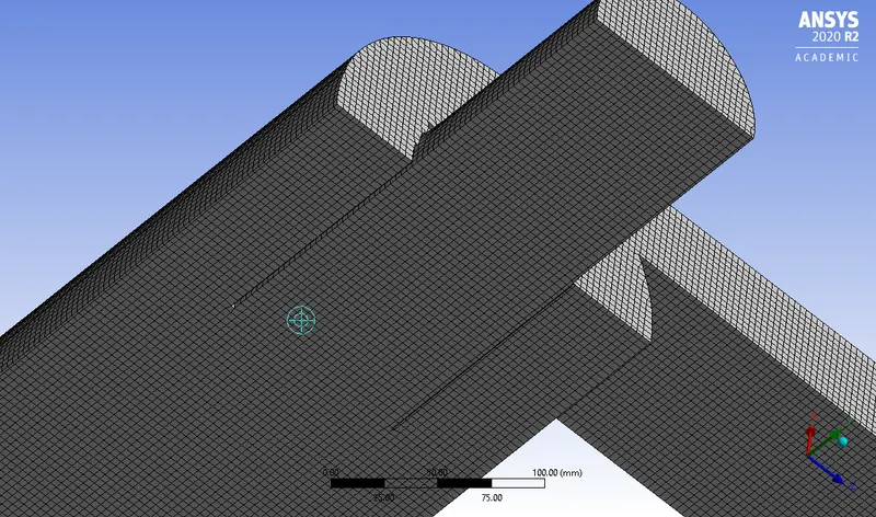
1. When we consider swirling flows, or simulations where we have to track particles and obtain the particle history data, it is important to have equally size mesh elements within the geometry.
2. Hence the cartesian mesh method was used to get equal volumes of mesh elements in the geometry.
3. The global size was chosen to be 20mm and the cartesian mesh size was set to be 5mm.
4. The total mesh count came out to be around 427k which is sufficient enough to track 300-400 particles
5. The mesh refinement plays a major role in deciding the total number of particles tracked.
6. If the mesh is too coarse, the number of particles may be very less, even below 10.
7. Hence, a fine mesh of 427k elements was produced and proceeded for case setup.

Setting up the case in Ansys Setup –

1. In this problem, the max velocity attained by the particles and air is very less as compared to the speed of sound.
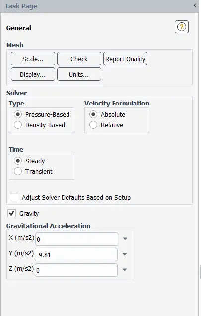
2. Hence, the Mach number is <<< 0.3. Hence, a pressure-based solver was used since density-based solvers are generally used for simulations with Mach no > 0.3.
3. In this particular simulation, a steady state solver was used since we do not require to observe each particle at every moment.
4. Observing the number of particles that have been trapped, escaped, and incomplete, is our main motive
5. Furthermore, a gravity value of 9.81 m/s^2 was added in the -ve Y direction.
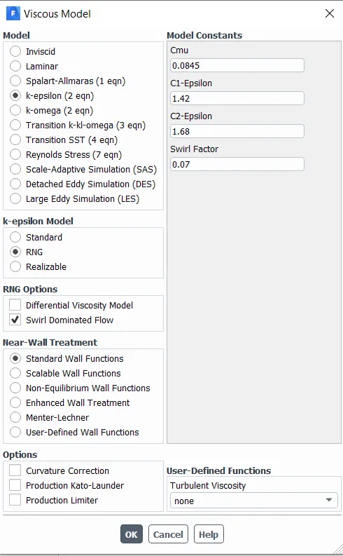
6. The K-epsilon RNG model was used in this particular problem.
7. This model is an upgradation of the standard k-epsilon model and is used mainly for swirling flows.
8. Moreover, the “swirl dominated flow” option was turned on for this simulation.
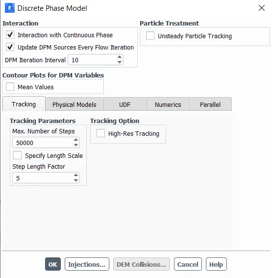
9. Afterwards, the discrete phase model option was turned and the settings were changed.
10. Here, the air particles represent the continuous phase whereas the solid particles represent the discontinuous phase.
11. These two phases can exchange mass and momentum within the flow.
12. Coupled Flow – The discrete phase can influence the flow of the continuous phase
13. Uncoupled Flow – The discrete phase will not have any interaction with the continuous phase
14. In this particular case, the particle size is very small, it doesn’t matter which option we chose.
15. The DPM interval was chosen as 10 and thus, the particle tracking data will be updated and showed on the console every 10 iterations.
16. The tracking parameters and specify length scale was set to default.
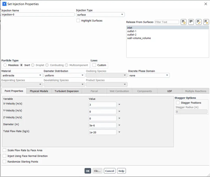
17. Then a new injection was created with the following parameters –

• Material – anthracite
• Particle type – inert
• Diameter distribution – uniform
• Injection type – surface
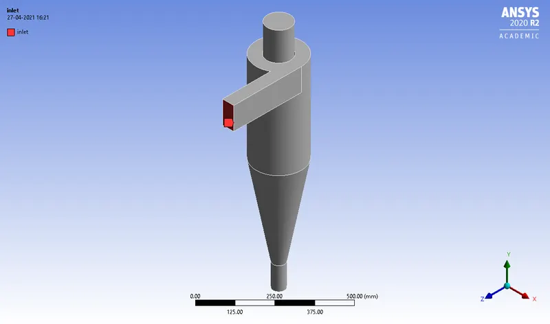
• Release from - INLET
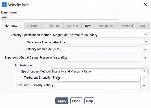
• Velocity – 1,3,5 m/s in the x direction
• Diameter of particles – 1,3,5 microns

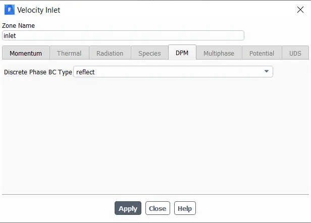
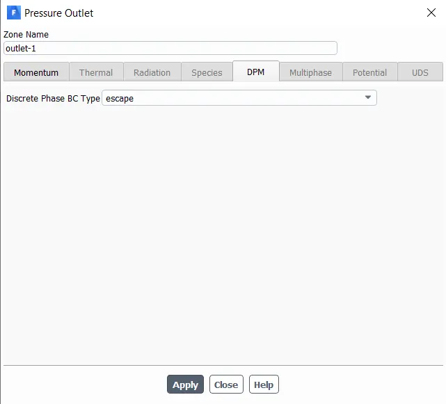
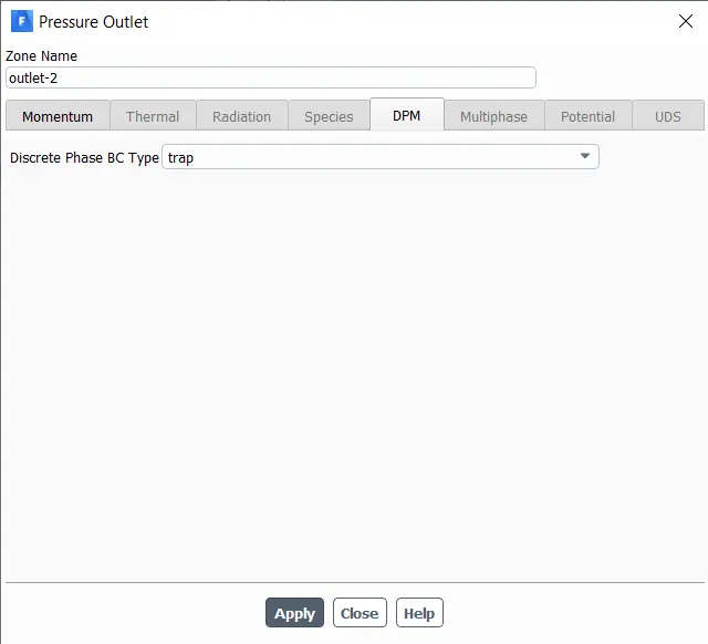
18. Furthermore, the boundary conditions for DPM were set accordingly

• Inlet – Reflect
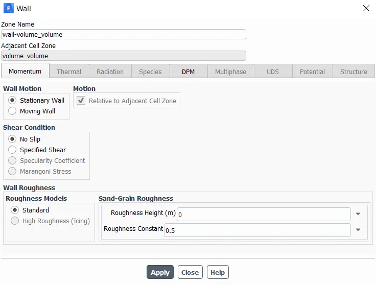
• Wall – Reflect
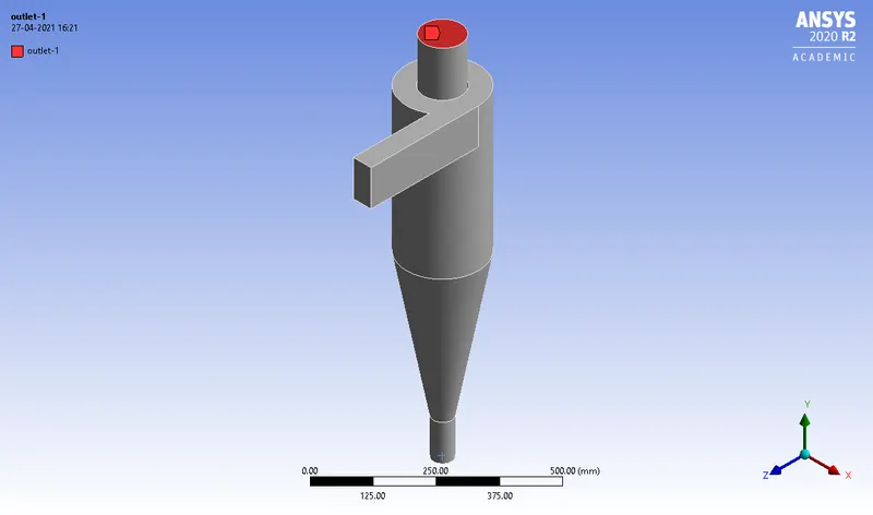
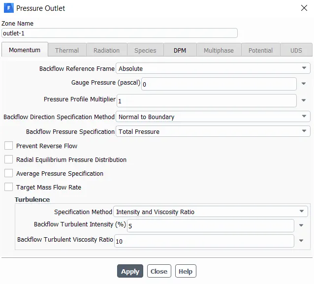
• Outlet top – escape
• Outlet Bottom – trap

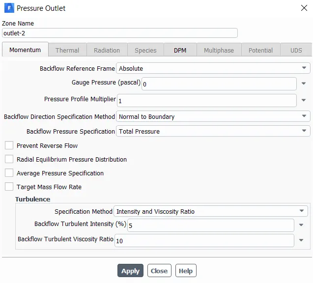
19. The inlet was set to a velocity inlet and outlet to a pressure outlet
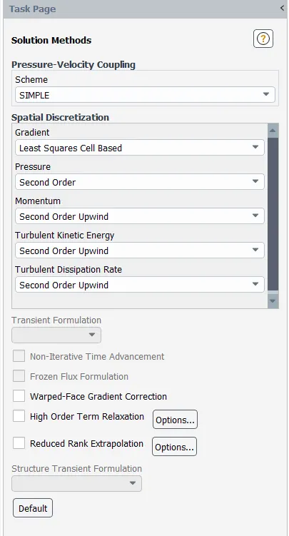
20. The coupled scheme with “second order upwind” was used for the turbulent kinetic energy and turbulent dissipation rate
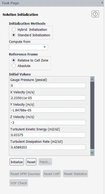
21. The solution was initialised using standard initialisation and was computed from inlet.
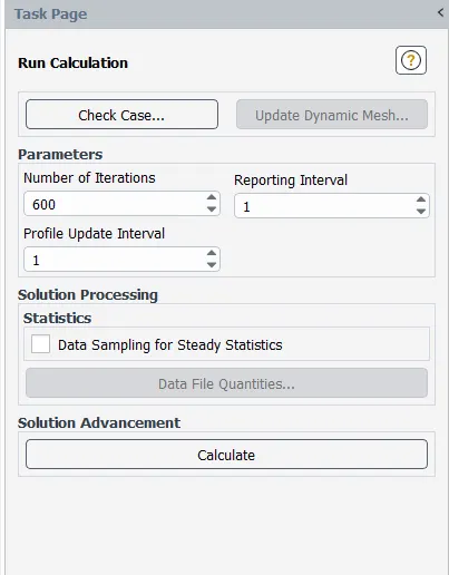
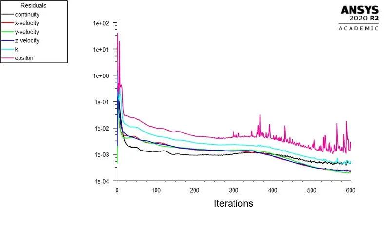
22. The problem was then run for 600 iterations and the results were observed

Results and findings –

1. Velocity = 3m/s, size = 5microns

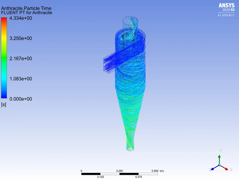
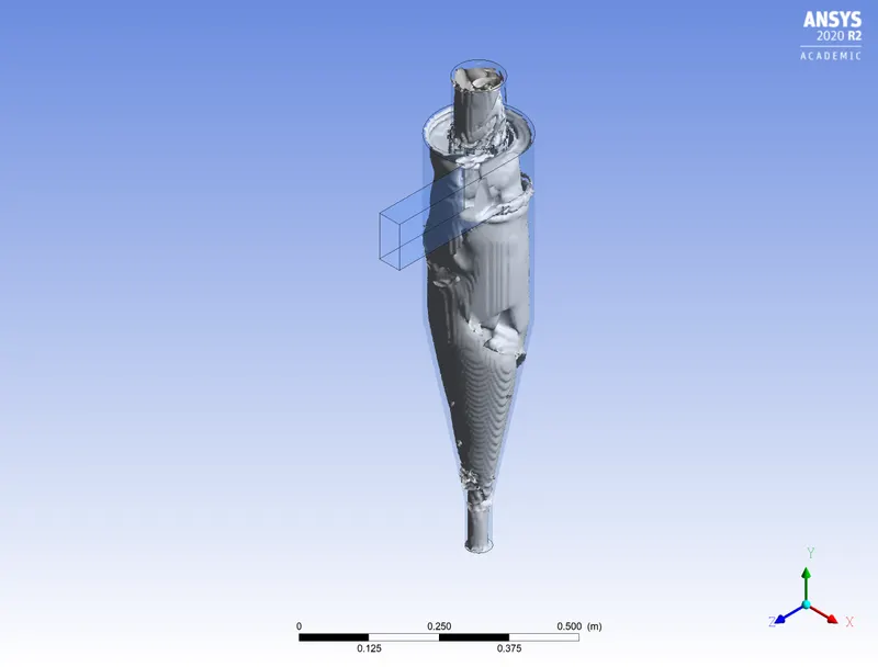
2. Velocity = 3m/s, size = 3microns

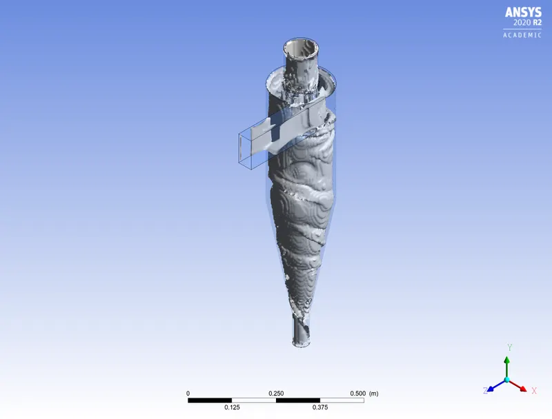
3. Velocity = 3m/s, size = 1microns

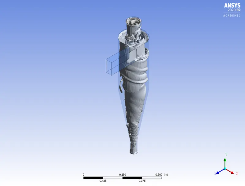
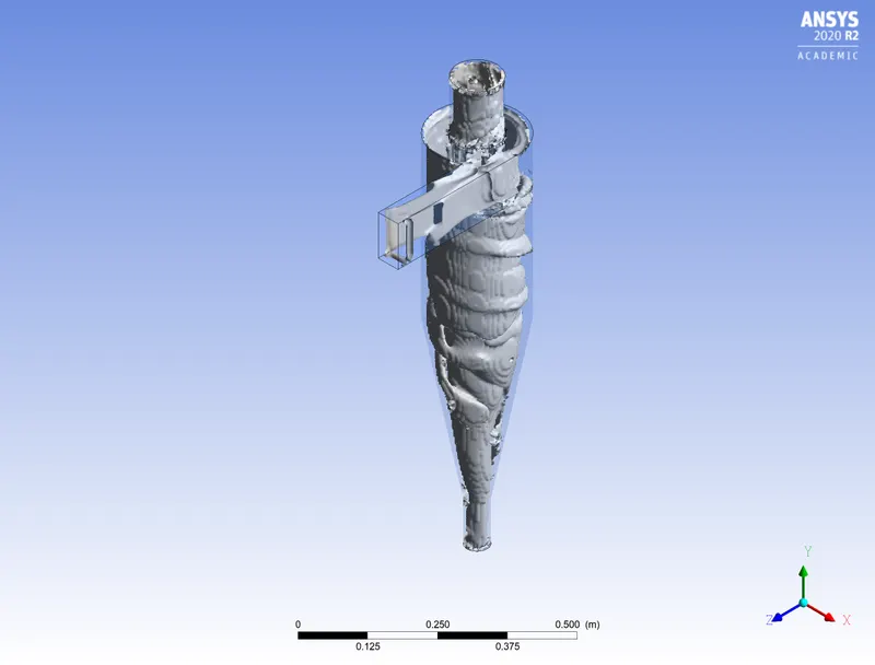
4. Velocity = 5m/s, size = 5microns

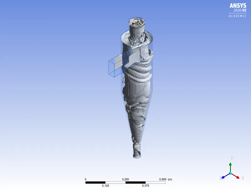
5. Velocity = 3m/s, size = 5microns

6. Velocity = 1m/s, size = 5microns

Conclusions and inferences –

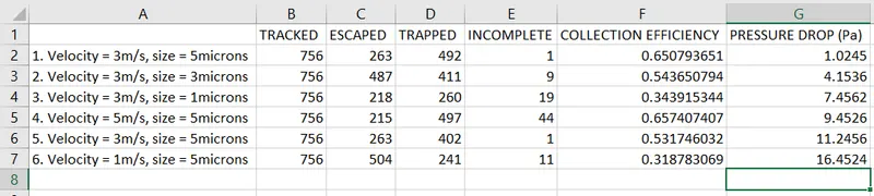
1. With increase in particle size at a constant fluid and particle velocity, the number of incomplete particles decreases.
2. With increase in particle size at a constant fluid and particle velocity, the collection efficiency increases
3. With increase in velocity at a constant particle size, the number of incomplete particles decreases.
4. With increase in velocity at a constant particle size, the collection efficiency increases

Reference research Papers -

1. https://www.sciencedirect.com/science/article/pii/S0307904X06000291

2. https://www.researchgate.net/publication/232747389_A_CFD_Study_on_the_Prediction_of_Cyclone_Collection_Efficiency