Week 7 - Simulation of a 1D Supersonic nozzle flow simulation using Macormack Method
Subsonic-supersonic nozzle:
The problem under consideration is the steady-state, isentropic flow through a convergent-divergent nozzle that can be shown by the following sketch.
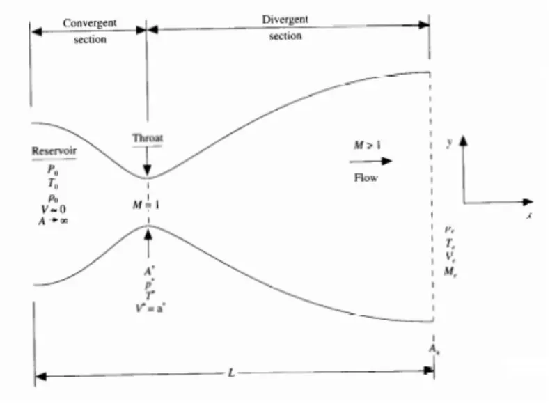
The variables in the diagram are described as follows:
P0, T0, ρ0, V0 are the Pressure, Temperature, Density, and Velocity at the inlet of the nozzle respectively.
A is the cross-sectional area at the reservoir (theoretical value tends to ∞).
M is the Mach number.
A’, P’, T’, and V’ are the Area, Pressure, Temperature, and Velocity at the throat respectively.
Pe, Te, Ve, and Me are the Pressure, Temperature, Velocity, and Mach number at the nozzle exit respectively.
The flow is supposed to be subsonic at the inlet region, sonic at the throat section, and supersonic at the divergent region.
The Governing Equations:
The governing equations of continuity, momentum conservation, and energy conservation for quasi-1D, steady-state, isentropic flow can be expressed as follows:
Continuity: ρ1v1A1=ρ2v2A2
Momentum: P1A1+ρ1v21A1+∫A2A1PdA=P2A2+ρ2v22A2
Energy: h1+v212=h2+v222
The subscripts 1 and 2 denote different locations along with the nozzle.
In our project, we are going to be solving the problem using 2 forms i.e., the conservative and the non-conservative forms of the governing equations. We use the normalized forms of these equations to make it easier to code these equations in MATLAB.
The normalized forms of the variables are as follows:
T1=TT0
ρ′=ρρ0
x′=xL
v′=va0
A′=AA⋅
Here, and are the temperature and density at the reservoir respectively. L is the length of the nozzle, a0 denotes the speed of sound in the reservoir and A* is the cross-sectional area at the throat section of the nozzle.
And then we compare and study the solutions obtained from both the forms of the equations. Both the forms of the governing equations are explained as follows:
Non-conservative form:
The non-conservative form of our governing equations for the given problem definition are as follows:
Continuity: ∂ρ′∂t′=−ρ∂v′∂x′−ρ′v′∂ln(A′)∂x′−v′∂ρ′∂x′
Momentum: ∂v′∂t′=−v′∂v′∂x′−1γ(∂T′∂x′+T′ρ′∂ρ′∂x′)
Energy: ∂T′∂t′=−V∂T′∂x′−(γ−1)T′[∂v′∂x′+v′∂lnA∂x′]
Conservative form:
The conservative form of our governing equations for the given problem definition are as follows:
Continuity: ∂∂t(ρA)+∂∂x(ρvA)=0
Momentum: ∂ρ′A′v′∂t′+∂ρ′A′(v′)2+(1/γ)P′A′∂x1=1γP′∂A′∂x′
Energy: ∂ρ′(e′γ−1+γ2(v′)2)A'∂t′+∂ρ′(e′r−1+γ2(V′)2)v'A'+P'A'v'∂x′=0
The above three equations are written in the form of solution vectors U, and the flux vectors F and the source term J, so that they are in a more generic form. Thus the U, F and J are written as follows:
U1=ρ1A1
U2=ρ1A1v1
U3=ρ′(eγ−1+γ2(v')2)A1
F1=ρ′A′v′
F2=ρ′A′v'2
F3=ρ′(e′γ−1+γ2(v′)2)v′A′+P′A′V′
J2=1γP′∂A′∂x′
And the original governing equations in the conservative form can be re-written as follows:
∂U1∂t′=−∂F1∂x′
∂U2∂t′=−∂F2∂x′+J2
∂U3∂t′=−∂F3∂x′
MacCormack’s technique:
MacCormack’s technique is an explicit finite difference technique that is second-order accurate. It is a variant of the Lax-Wendroff method but a lot simpler in the application.
MacCormack’s is a two-step predictor-corrector sequence with forward differences for the spatial derivatives in the predictor step and the backward differences for the spatial derivatives in the corrector step. The exact method is to first obtain the forward differences for the spatial derivatives in the predictor step for all the grid points in a particular time step and then to obtain the predicted values for all the primitive variables from the first two terms of a Taylor series. Then, the backward difference of the previously obtained predicted values is obtained in the corrector step.
Once the predictor-corrector steps are obtained, the final values for all the primitive variables for the equations being solved are obtained by taking the average of the values obtained from both the predictor and the corrector steps.
We are calculating both the predictor and the corrector values and then taking the average of the two so that the final solution obtained is second-order accurate. Otherwise, with either just the predictor step or with just the corrector step, the solution would just be only first-order accurate.
Program to simulate the isentropic flow through a quasi 1D subsonic-supersonic nozzle in MATLAB:
Following is the main function:
clear all
close all
clc

%Initialising the profile length
l = 3;

%Defining the number of nodes
n = 31;

%Defining the grid space
x = linspace(0,l,n);

%Initialising the number of time-steps.
nt = 1000;

%Function call for the non-conservative form.
[rho_nc,t_nc,v_nc,mfr_nc,p_nc,mach_nc,rho_t_nc,t_t_nc,v_t_nc,mfr_t_nc,p_t_nc,mach_t_nc] = non_conservative(n,nt,l);

%Function call for the conservative form.
[rho_c,t_c,v_c,mfr_c,p_c,mach_c,rho_t_c,t_t_c,v_t_c,mfr_t_c,p_t_c,mach_t_c] = conservative(n,nt,l);

%Plotting to compare the mass flow rate for conservative vs non-conservative forms.
figure(9)
plot(x,mfr_nc,'color','r')
hold on
plot(x,mfr_c,'color','b')
legend('Non-conservative','Conservative')
title('Comparision of Mass flow rates in Conservative vs Non-Conservative forms.')
Following is the function for Non-conservative form:
function[rho_nc,t_nc,v_nc,mfr_nc,p_nc,mach_nc,rho_t_nc,t_t_nc,v_t_nc,mfr_t_nc,p_t_nc,mach_t_nc] = non_conservative(n,nt,l)

%Defining the node points
x = linspace(0,l,n);
%Defining delta x
dx = x(2) - x(1);

%Defining initial values for density, temperature and velocity
rho = 1 - 0.3146*x;
T = 1 - 0.2314*x;
v = (0.1 + 1.09*x).*T.^0.5;

%Defining specific heat ratio
gamma = 1.4;

%Defining area at all node points
a = 1 + 2.2 * (x - 1.5).^2;

%Defining Courant number
c = 0.5;

%Calculating the node point at throat section.
x_t = find(a==1);

%Starting time loop.
for k = 1:nt

    %Defining the value for dt according to the courant number formula.
    dt = min((c.*dx)./(a+v));

    %Saving the initial values
    rho_old = rho;
    v_old = v;
    T_old = T;

    %Starting the loop for predictor step.
    for j = 2:n-1

    %Defining the derivatives for future simplifications
    dvdx = (v(j+1) - v(j))/dx;
    drhodx = (rho(j+1) - rho(j))/dx;
    dtdx = (T(j+1) - T(j))/dx;
    dlog_a_dx = (log(a(j+1)) - log(a(j)))/dx;

    %Solving for the mass, momentum and energy conservation equations at each grid point in predictor step.
    drhodt_p(j) = (-rho(j) * dvdx) - ((rho(j) * v(j)) * dlog_a_dx) - (v(j) * (drhodx));

    dvdt_p(j) = (-v(j) * (dvdx)) - ((1/gamma) * (dtdx + (T(j)/rho(j)) * (drhodx)));

    dtdt_p(j) = (-v(j) * (dtdx)) - (gamma - 1) * T(j) * (dvdx + (v(j) * dlog_a_dx));

    %Updating the values for each grid point in the predictor step.
    v(j) = v(j) + dvdt_p(j) * dt;
    rho(j) = rho(j) + drhodt_p(j) * dt;
    T(j) = T(j) + dtdt_p(j) * dt;

    end

    %Starting the loop for the corrector step.
    for j = 2:n-1

    %Defining derivatives for simplification.
    dvdx = (v(j) - v(j - 1))/dx;
    drhodx = (rho(j) - rho(j - 1))/dx;
    dtdx = (T(j) - T(j - 1))/dx;
    dlog_a_dx = (log(a(j)) - log(a(j - 1)))/dx;

    %Solving for the mass, momentum and energy conservation in the corrector step.
    drhodt_c(j) = (-rho(j) * dvdx) - ((rho(j) * v(j)) * dlog_a_dx) - (v(j) * (drhodx));

    dvdt_c(j) = (-v(j) * (dvdx)) - ((1/gamma) * (dtdx + (T(j)/rho(j)) * (drhodx)));

    dtdt_c(j) = (-v(j) * (dtdx)) - (gamma - 1) * T(j) * (dvdx + (v(j) * dlog_a_dx));

    end

    %Calculating the average of predictor and corrector steps.
    dvdt = 0.5*(dvdt_p + dvdt_c);
    drhodt = 0.5*(drhodt_p + drhodt_c);
    dtdt = 0.5 * (dtdt_p + dtdt_c);

    %Solution update for the next iteration in time-step.
    for i = 2:n-1

        rho(i) = rho_old(i) + drhodt(i) * dt;
        v(i) = v_old(i) + dvdt(i) * dt;
        T(i) = T_old(i) + dtdt(i) * dt;

    end

    %Assigning values to variables that is returned to the main function.
    rho_nc = rho;
    t_nc = T;
    v_nc = v;

    %Defining initial conditions at inlet.
    v(1) = 2 * v(2) - v(3);

    %Defining initial conditions at outlet.
    v(n) = 2 * v(n-1) - v(n-2);
    rho(n) = 2 * rho(n-1) - rho(n-2);
    T(n) = 2 * T(n-1) - T(n-2);

    %Calculating mass flow rate, pressure and mach number for the present time-step.
    mfr_nc = rho_nc .* a .* v_nc;
    p_nc = rho_nc .* t_nc;
    mach_nc = (v_nc./sqrt(t_nc));

    %Calculating the variables at the throat section for the present time-step.
    rho_t_nc(k) = rho_nc(x_t);
    t_t_nc(k) = t_nc(x_t);
    v_t_nc(k) = v_nc(x_t);

    mfr_t_nc(k) = mfr_nc(x_t);
    p_t_nc(k) = p_nc(x_t);
    mach_t_nc(k) = mach_nc(x_t);

    %plotting for variation of mass flow rate distribution at different time-steps.
    figure(1)
    if k == 1
        plot(x,mfr_nc,'color','r','linewidth',2);
        hold on

    elseif k == 50
        plot(x,mfr_nc,'color','b','linewidth',2);
        hold on

    elseif k == 100
        plot(x,mfr_nc,'color','g','linewidth',2);
        hold on

    elseif k == 400
        plot(x,mfr_nc,'color','k','linewidth',2);
        hold on

    elseif k == 700
        plot(x,mfr_nc,'color','c','linewidth',2);
        hold on

    elseif k == 1000
        plot(x,mfr_nc,'color','m','linewidth',2);
        hold on


    end

    xlabel('Profile Length');
    ylabel('Mass Flow Rate');
    title('NON-CONSERVATIVE FORM. Mass Flow Rates at different time-steps.');
    legend('nt = 1','nt = 50','nt = 100','nt = 400','nt = 700','nt = 1000','nt = 1400');

    %Plotting for time wise vatiation of primitive variables at each iteration.
    figure(2)

    subplot(2,3,1)
    plot(x,rho_nc)
    xlabel('Profile Length')
    ylabel('Density')

    subplot(2,3,2)
    plot(x,t_nc)
    xlabel('Profile Length')
    ylabel('Temperature')
    title(sprintf('NON_CONSERVATIVE: Time wise variation of primitive variables. Time step = %s',num2str(k)));

    subplot(2,3,3)
    plot(x,v_nc)
    xlabel('Profile Length')
    ylabel('Velocity')

    subplot(2,3,4)
    plot(x,mfr_nc)
    xlabel('Profile Length')
    ylabel('Mass Flow Rate')
    axis([0 3 0 2])

    subplot(2,3,5)
    plot(x,p_nc)
    xlabel('Profile Length')
    ylabel('Pressure')

    subplot(2,3,6)
    plot(x,mach_nc)
    xlabel('Profile Length')
    ylabel('Mach Number')

    M(k) = getframe(gcf);

    pause(0.003);

end

movie(M)
videofile = VideoWriter('non_conservative.mp4');
open(videofile)
writeVideo(videofile,M)
close(videofile)

%Plotting for time wise variation of primitive variables.
figure(3)
subplot(5,1,1)
plot(linspace(1,nt,n),rho_nc)
xlabel('Time Step')
ylabel('Density')
title({'NON-CONSERVATIVE';'Time wise variation of Density'})

subplot(5,1,2)
plot(linspace(1,nt,n),t_nc)
xlabel('Time Step')
ylabel('Temperature')
title('Time wise variation of Temperature')

subplot(5,1,3)
plot(linspace(1,nt,n),v_nc)
xlabel('Time Step')
ylabel('Velocity')
title('Time wise variation of Velocity')

subplot(5,1,4)
plot(linspace(1,nt,n),p_nc)
xlabel('Time Step')
ylabel('Pressure')
title('Time wise variation of Pressure')

subplot(5,1,5)
plot(linspace(1,nt,n),mach_nc)
xlabel('Time Step')
ylabel('Mach Number')
title('Time wise variation of Mach Number')

%Plotting for time wise variation of primitive variables at throat section.
figure(4)
subplot(5,1,1)
plot(linspace(1,nt,nt),rho_t_nc)
xlabel('Time Step')
ylabel('Density')
title({'NON-CONSERVATIVE';'Time wise variation of Density at throat'})

subplot(5,1,2)
plot(linspace(1,nt,nt),t_t_nc)
xlabel('Time Step')
ylabel('Temperature')
title('Time wise variation of Temperature at throat')

subplot(5,1,3)
plot(linspace(1,nt,nt),v_t_nc)
xlabel('Time Step')
ylabel('Velocity')
title('Time wise variation of Velocity at throat')

subplot(5,1,4)
plot(linspace(1,nt,nt),p_t_nc)
xlabel('Time Step')
ylabel('Pressure')
title('Time wise variation of Pressure at throat')

subplot(5,1,5)
plot(linspace(1,nt,nt),mach_t_nc)
xlabel('Time Step')
ylabel('Mach Number')
title('Time wise variation of Mach Number at throat')

end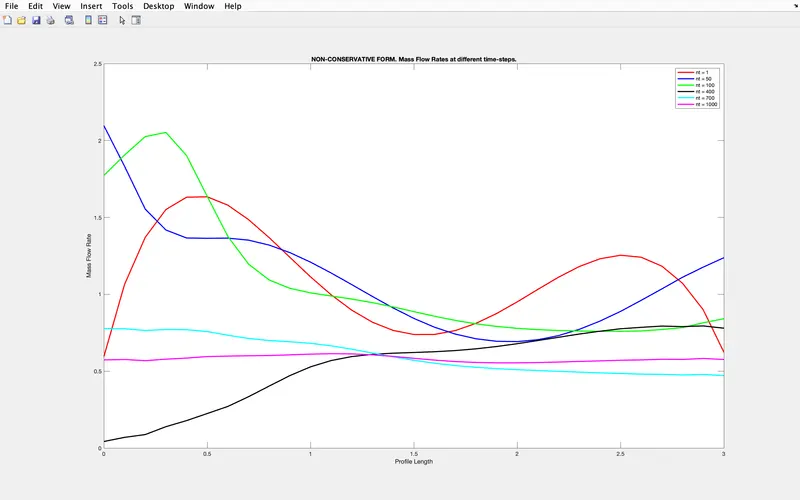
Following is the function for the conservative form:
function [rho_c,t_c,v_c,mfr_c,p_c,mach_c,rho_t_c,t_t_c,v_t_c,mfr_t_c,p_t_c,mach_t_c]=conservative(n,nt,l)

%Defining the gird points of the domain
x=linspace(0,l,n);
%Defining delta x
dx=x(2)-x(1);
%initializing gamma value
gama=1.4;
%Defining area at all node points
a=1+2.2*(x-1.5).^2;
%Calculating the node number of the throat
x_t = find(a==1);

%Defining the intial conditions
for i=1:length(x)
    if x(i)>= 0 && x(i)<= 0.5
        rho_c(i)=1;
        t_c(i)=1;
    elseif x(i)>=0.5 && x(i)<=1.5
        rho_c(i)=1-0.366*(x(i)-0.5);
        t_c(i)=1-0.167*(x(i)-0.5);
    elseif x(i)>=1.5 && x(i)<= 3.0
        rho_c(i)=0.634-0.3879*(x(i)-1.5);
        t_c(i)=0.833-0.3507*(x(i)-1.5);
    end
end

%Calcualting velocity and pressure from the fixed intial conditions
v_c=0.59./(rho_c.*a);
p_c=rho_c.*t_c;

%Calculating initial solution vectors
u1=rho_c.*a;
u2=rho_c.*a.*v_c;
u3=rho_c.*a.*(t_c./(gama-1)+(gama/2).*v_c.^2);

%Calculating time step size calulation based on courant number
c=0.5;
dt=min(c.*dx./(sqrt(t_c)+v_c));

%Starting the time loop
for k=1:nt

    %Saving the intial values
    u1_old=u1;
    u2_old=u2;
    u3_old=u3;

    %Calculating the Flux vectors from the initial solution vector
    f1=u2;
    f2=(u2.^2./u1)+((gama-1)/(gama)*(u3-(gama*u2.^2)./(2*u1)));
    f3=((gama*u2.*u3)./u1)-((gama*(gama-1))/2)*((u2.^3)./(u1.^2));

    %Starting the loop for predictor step
    for j=2:n-1

        %Defining the source term
        j2(j)=(1/gama)*rho_c(j)*t_c(j)*((a(j+1)-a(j))/dx);

        df1dx=(f1(j+1)-f1(j))/dx;
        df2dx=(f2(j+1)-f2(j))/dx;
        df3dx=(f3(j+1)-f3(j))/dx;

        %Solving for the mass, momentum and the energy conservation equations in the predictor step.
        du1dt_p(j)=-df1dx;
        du2dt_p(j)=-df2dx+j2(j);
        du3dt_p(j)=-df3dx;

        %Solution vectors are updated after prdictor step
        u1(j)=u1(j)+du1dt_p(j)*dt;
        u2(j)=u2(j)+du2dt_p(j)*dt;
        u3(j)=u3(j)+du3dt_p(j)*dt;
    end

    %Calculting primitive variables from the predictor solution vectors
    rho_c=u1./a;
    v_c=u2./u1;
    t_c=(gama-1)*(u3./u1-(gama/2)*v_c.^2);
    p_c=rho_c.*t_c;

    %Defining the boundary conditions at inlet
    u1(1)=rho_c(1).*a(1);
    u2(1)=(2*u2(2))-u2(3);
    u3(1)=u1(1)*(t_c(1)/(gama-1)+(gama/2)*(u2(1)/u1(1))^2);

    %Defining the boundary conditions at outlet
    u1(n)=2*u1(n-1)-u1(n-2);
    u2(n)=2*u2(n-1)-u2(n-2);
    u3(n)=2*u3(n-1)-u3(n-2);

    %Updating the flux vectors from the predictor solution vectors
    f1=u2;
    f2=((u2.^2)./u1)+((gama-1)/gama)*(u3-((gama*u2.^2)./(2*u1)));
    f3=(gama*u2.*u3./u1)-(gama*(gama-1)/2)*(u2.^3./u1.^2);

    %Starting the loop for the corrector step
    for j=2:n-1

        %Defining the source term
        j2(j)=(1/gama)*rho_c(j)*t_c(j)*((a(j)-a(j-1))/dx);

        df1dx=(f1(j)-f1(j-1))/dx;
        df2dx=(f2(j)-f2(j-1))/dx;
        df3dx=(f3(j)-f3(j-1))/dx;

        %Solving for mass, momentum and energy conservation equations in the corrector step.
        du1dt_c(j)=-df1dx;
        du2dt_c(j)=-df2dx+j2(j);
        du3dt_c(j)=-df3dx;

    end

        %Taking the average of predictor and the corrector steps.
        du1dt=0.5*(du1dt_p+du1dt_c);
        du2dt=0.5*(du2dt_p+du2dt_c);
        du3dt=0.5*(du3dt_p+du3dt_c);

        %final solution update
        for mach_c=2:n-1
        u1(mach_c)=u1_old(mach_c)+du1dt(mach_c)*dt;
        u2(mach_c)=u2_old(mach_c)+du2dt(mach_c)*dt;
        u3(mach_c)=u3_old(mach_c)+du3dt(mach_c)*dt;
        end

        %Boundary conditions at inlet
        u1(1)=rho_c(1).*a(1);
        u2(1)=(2*u2(2))-u2(3);
        u3(1)=u1(1)*(t_c(1)/(gama-1)+(gama/2)*(u2(1)/u1(1))^2);

        %Boundary conditions at outlet
        u1(n)=2*u1(n-1)-u1(n-2);
        u2(n)=2*u2(n-1)-u2(n-2);
        u3(n)=2*u3(n-1)-u3(n-2);


    %Calculating the primitive variables from the solution vectors
    rho_c=u1./a;
    v_c=u2./u1;
    t_c=(gama-1)*((u3./u1)-(gama/2)*v_c.^2);
    p_c=rho_c.*t_c;


    %mach no calculation
    mach_c=(v_c)./(t_c.^0.5);
    %mass flow rate calculation
    mfr_c=rho_c.*v_c.*a;

    %plotting for variation of mass flow rate distribution at different time-steps.
    figure(5)

    if k == 1
        plot(x,mfr_c,'color','r','linewidth',2);
        hold on

    elseif k == 50
        plot(x,mfr_c,'color','b','linewidth',2);
        hold on

    elseif k == 100
        plot(x,mfr_c,'color','g','linewidth',2);
        hold on

    elseif k == 400
        plot(x,mfr_c,'color','k','linewidth',2);
        hold on

    elseif k == 700
        plot(x,mfr_c,'color','c','linewidth',2);
        hold on

    elseif k == 1000
        plot(x,mfr_c,'color','m','linewidth',2);
        hold on

    end

    hold on
    xlabel('Profile Length');
    ylabel('Mass Flow Rate');
    title('CONSERVATIVE FORM. Mass Flow Rates at different time-steps.');
    legend('nt = 1','nt = 50','nt = 100','nt = 400','nt = 700','nt = 1000','nt = 1400');

    %Plotting for time wise vatiation of primitive variables at each iteration.
    figure(6)

    subplot(2,3,1)
    plot(x,rho_c)
    xlabel('Profile Length')
    ylabel('Density')

    subplot(2,3,2)
    plot(x,t_c)
    xlabel('Profile Length')
    ylabel('Temperature')
    title(sprintf('CONSERVATIVE: Time wise variation of primitive variables. Time step = %s',num2str(k)));

    subplot(2,3,3)
    plot(x,v_c)
    xlabel('Profile Length')
    ylabel('Velocity')

    subplot(2,3,4)
    plot(x,mfr_c)
    xlabel('Profile Length')
    ylabel('Mass Flow Rate')
    axis([0 3 0 2])

    subplot(2,3,5)
    plot(x,p_c)
    xlabel('Profile Length')
    ylabel('Pressure')

    subplot(2,3,6)
    plot(x,mach_c)
    xlabel('Profile Length')
    ylabel('Mach Number')

    M(k) = getframe(gcf);

    pause(0.003);


%saving the throat values of primitive variables for different time steps
t_t_c(k)=t_c(x_t);
p_t_c(k)=p_c(x_t);
rho_t_c(k)=rho_c(x_t);
mach_t_c(k)=mach_c(x_t);
v_t_c(k) = v_c(x_t);
mfr_t_c(k) = mfr_c(x_t);

end

movie(M)
videofile = VideoWriter('conservative.mp4');
open(videofile)
writeVideo(videofile,M)
close(videofile)

%Plotting for time wise variation of primitive variables.
figure(7)
subplot(5,1,1)
plot(linspace(1,nt,n),rho_c)
xlabel('Time Step')
ylabel('Density')
title({'CONSERVATIVE';'Time wise variation of Density'})

subplot(5,1,2)
plot(linspace(1,nt,n),t_c)
xlabel('Time Step')
ylabel('Temperature')
title('Time wise variation of Temperature')

subplot(5,1,3)
plot(linspace(1,nt,n),v_c)
xlabel('Time Step')
ylabel('Velocity')
title('Time wise variation of Velocity')

subplot(5,1,4)
plot(linspace(1,nt,n),p_c)
xlabel('Time Step')
ylabel('Pressure')
title('Time wise variation of Pressure')

subplot(5,1,5)
plot(linspace(1,nt,n),mach_c)
xlabel('Time Step')
ylabel('Mach Number')
title('Time wise variation of Mach Number')

%Plotting for time wise variation of primitive variables at throat section.
figure(8)
subplot(5,1,1)
plot(linspace(1,nt,nt),rho_t_c)
xlabel('Time Step')
ylabel('Density')
title({'CONSERVATIVE';'Time wise variation of Density at throat'})

subplot(5,1,2)
plot(linspace(1,nt,nt),t_t_c)
xlabel('Time Step')
ylabel('Temperature')
title('Time wise variation of Temperature at throat')

subplot(5,1,3)
plot(linspace(1,nt,nt),v_t_c)
xlabel('Time Step')
ylabel('Velocity')
title('Time wise variation of Velocity at throat')

subplot(5,1,4)
plot(linspace(1,nt,nt),p_t_c)
xlabel('Time Step')
ylabel('Pressure')
title('Time wise variation of Pressure at throat')

subplot(5,1,5)
plot(linspace(1,nt,nt),mach_t_c)
xlabel('Time Step')
ylabel('Mach Number')
title('Time wise variation of Mach Number at throat')

end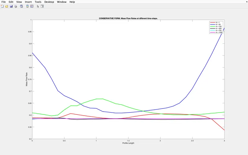
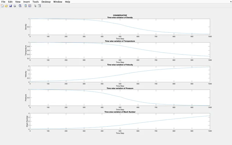
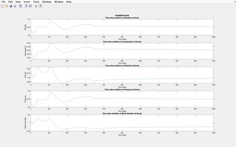
Conservative vs Non-conservative forms of solutions:
For a general understanding, the conservative form that the Euler's approach where the control volume is fixed and the properties of the fluid elements passing through it are studied. Whereas, the non-conservative form takes the Lagrangian approach where certain fluid elements and their properties are studied along its path in the overall control domain. This gives an advantage to the conservative form in cases where there are sudden shocks in the domain where the system of variables would undergo a very significant change in the consecutive spatial domain.
Although both the forms make no difference when we approach the problem analytically, there is a significant difference when we look at the coding aspect of the problem. In non-conservative form, the solution is calculated based directly on the primitive variables whereas, in the conservative form, the solutions are obtained from the unit vectors and the flux vectors. This would mean that the solutions are obtained at a much higher accuracy in the non-conservative form, whereas in the conservative form, there is a good chance of the solution not blowing up in the conservative form.
Essentially, both methods have their own advantages and disadvantages over the other. Hence, choosing one method over the other requires a very good understanding of the problem under consideration.
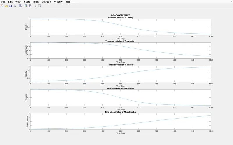
In our problem, we could see that the solutions converged a lot faster using the conservative form. The plot below shows the normalized Mass Flow Rate obtained in both the conservative form and the non-conservative form:
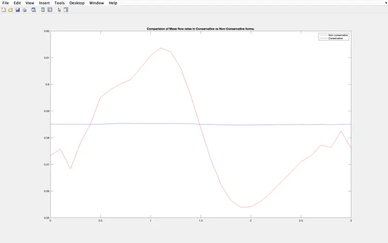
Here, in our specific case, we can conclude that the conservative form has also lead to a more accurate solution because the solution obtained is closer to the analytical solution when compared with the non-conservative solution.
Grid Independence test:
In general, when we perform any calculations using numerical methods, we calculate our governing equations across fixed node points. These node points essentially form a grid/mesh. As the number of nodes increases, the spatial difference between the points decreases and the solution obtained is more accurate. But this in turn, increases the overall computation time. Hence, it is very important to arrive at a value for the number of nodes or basically, the mesh density for our physical domain under consideration so that we can estimate the solution to be within the acceptable range of accuracy and save our computation time by not considering mesh with higher densities.
| Density | Temperature | Pressure | Mach Number | |
| Analytical solution | 0.634 | 0.833 | 0.528 | 1 |
| 61 nodes - conservative | 0.639 | 0.8355 | 0.5339 | 0.9979 |
| 61 nodes - non conservative | 0.5917 | 0.8081 | 0.4782 | 1.0753 |
| 31 nodes - conservative | 0.6517 | 0.8407 | 0.5479 | 0.9792 |
| 31 nodes - non conservative | 0.5961 | 0.8136 | 0.485 | 1.0867 |
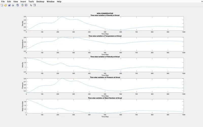
Our code was run again with 61 node points and the above table gives us a picture of how the solutions obtained compare with the actual analytical solution. The values are that of the primitive variables in the throat section of our domain. The analytical were obtained with reference from the textbook "Computational Fluid Dynamics by John D Anderson."
It becomes quite obvious that a higher number of nodes lead to a solution that is more accurate. But, the solutions obtained from the mesh with 31 nodes were also reasonably accurate. Hence, one can decide if one wants a higher accuracy that would take more computational time or stop at a lower mesh density with a slight compromise on the solution accuracy.