Project 2 - Rankine cycle Simulator

AIM: Create a Rankine cycle stimulator using MATLAB.

OBJECTIVE:

• Calculate each points of the rankine cycle.
• Plot T-S & H-S diagram for those values.
• Calculatethe efficiency.

THEORY:

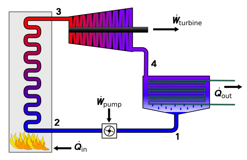
The Rankine cycle closely describes the process by which steam engines commonly found in thermal power generation plants harness the thermal energy of a fuel or other heat source to generate electricity. Possible heat sources include combustion of fossil fuels such as coal, natural gas, or oil, renewable fuels like biomass or ethanol, nuclear fission, and concentrated solar power. Common heat sinks include ambient air above or around a facility and bodies of water such as rivers, ponds, and oceans.

The ability of a Rankine engine to harness energy depends on the relative temperature difference between the heat source and heat sink. The greater the differential, the more mechanical power can be efficiently extracted out of heat energy, as per Carnot's theorem.

The efficiency of the Rankine cycle is limited by the high heat of vaporization of the working fluid. Unless the pressure and temperature reach super critical levels in the boiler, the temperature range that the cycle can operate over is quite small: Steam turbine entry temperatures are typically around 565 °C and condenser temperatures are around 30 °C. This gives a theoretical maximum Carnot efficiency for the turbine alone of about 63.8% compared with an actual overall thermal efficiency of less than 50% for typical power stations. This low steam turbine entry temperature (compared to a gas turbine) is why the Rankine (steam) cycle is often used as a bottoming cycle to recover otherwise rejected heat in combined-cycle gas turbine power stations.

Rankine engines generally operate in a closed loop where the working fluid is reused. The water vapour with condensed droplets often seen billowing from power stations is created by the cooling systems (not directly from the closed-loop Rankine power cycle). This 'exhaust' heat is represented by the "Q_out" flowing out of the lower side of the cycle shown in the T–s diagram below. Cooling towers operate as large heat exchangers by absorbing the latent heat of vaporization of the working fluid and simultaneously evaporating cooling water to the atmosphere.

The four processes in the Rankine cycle

There are four processes in the Rankine cycle. The states are identified by numbers (in brown) in the T–s diagram.

• Process 1–2: The working fluid is pumped from low to high pressure. As the fluid is a liquid at this stage, the pump requires little input energy. Process 1-2 is isentropic compression.
• Process 2–3: The high-pressure liquid enters a boiler, where it is heated at constant pressure by an external heat source to become a dry saturated vapour. The input energy required can be easily calculated graphically, using an enthalpy–entropy chart (h–s chart, or Mollier diagram), or numerically, using steam tables or software. Process 2-3 is constant pressure heat addition in boiler.
• Process 3–4: The dry saturated vapour expands through a turbine, generating power. This decreases the temperature and pressure of the vapour, and some condensation may occur. The output in this process can be easily calculated using the chart or tables noted above. Process 3-4 is isentropic expansion.
• Process 4–1: The wet vapour then enters a condenser, where it is condensed at a constant pressure to become a saturated liquid. Process 4-1 is constant pressure heat rejection in condenser.

PROCEDURE:

• The program begins with the clear all, close all, clc to erase the workspace and plots.
• Input variables p1,T1,p2 are given. At the state point 1, values for the enthalpy and entropy are extracted as a function of pressure and temperature.
• h_pT,s_pT,hL_p,sV_p etc are the default variables whose value is stored in XSteam function file.
• Similarly, all the variables for all the points are extracted using a suitable format.
• Pressure, temperature, entropy, enthalpy for all the state points are extracted as a function of the dependent variable from the XSteam file.
• Ate the state point 2 is a condenser inlet where the high-pressure steam is converted into low-pressure water and hence dryness fraction, enthalpy and entropy for the saturated vapour and saturated water are considered to calculate the specific enthalpy.
• Ate stae point 3 the water is condensed back to its saturation temperature and fed to the pump, this temperature of the water at the exit ofg the condenser and entry to the pump is same.
• At state point 4 this is constant pressure hat addition, hence pressure is equal to p1, but yhe temperature increases on heating at constant pressure and constant volume as our entropy same and hence cp/cv=gamma is considered to find the temperature T4.
• Define two more points 5 and 6 to plot the cycle n detail,
• Work done, heat evolved and efficiency are calculated by the formulae.
• To plot the saturation curve the temperature range is defined using linspace command and for the overall length of this temperature values of enthalpy and entropy are calculated at every temperature point. The break in the saturation curve seperates the liquid phase and vapour phase.
• Now all the necessary data is found out, plotting is done for both T-S & H-S curves using the plot commands and annotations are assigned using text command.
• Results of the cycle simulation is displayed over command window using fprintf command.

CODE:

close all
clear all
clc

%Rankine Cycle
%process
fprintf('Rankine Cycle')
fprintf('1-2 isobaric heat transfern')
fprintf('2-3 isentropic expansionn')
fprintf('3-4 isobaric heat rejectionn')
fprintf('4-1 isentropic compressionn')

%inputs
p1 = 30;  
T1 = 400; 
p2 = 0.05; 

%calculation at each point
%state point 1
h1 = XSteam('h_pt',p1,T1);
s1 = XSteam('s_pt',p1,T1);

%state point 2
s2 = s1;
sf2 = XSteam('sL_p',p2);
sg2 = XSteam('sV_p',p2);
hf2 = XSteam('hL_p',p2);
hg2 = XSteam('hV_p',p2); %x2 = (s2-sf2)/(sg2-sf2)
s2 = sg2;
h2 = hg2;                 %hf2 +(x2*(hg2-hf2))
T2 = XSteam('T_hs',h2,s2);

%state point 3
T3=T2;
p3 = p2;
s3 = XSteam('sL_T',T3);
h3 = XSteam('hL_T',T3);
v3 = XSteam('vL_p',p2);

%state point 4
p4 = p1;
s4 = s3;
Cp4 = XSteam('Cp_ps',p4,s4);
Cv4 = XSteam('Cv_ps',p4,s4);
gamma = Cp4/Cv4;
r = (gamma-1)/gamma;
T4 = T3*(p4/p3)^r;

%other values
Wt = h1-h2;  %turbine work
Wp = v3*(p1-p2)*100;  %pump work
h4= Wp+h3;
W_net = Wt-Wp;
Qs = h1-h4;
N_per = (W_net/Qs)*100;
steam_rate = 3600/(Wt-Wp);

%points help in plotting
T5 =XSteam('Tsat_p',p1);
T6 = T5;
s5 = XSteam('sL_p',p1);
s6 = XSteam('sV_p',p1);
h5 = XSteam('hL_p',p1);
h6 = XSteam('hV_p',p1);

%printing all stae posint
fprintf('n---------RESULTS--------n')
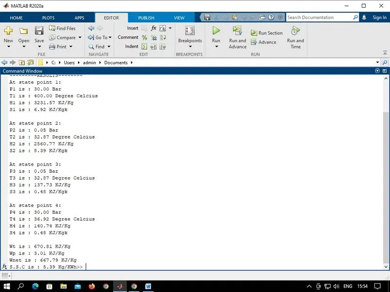
fprintf('At state point 1:nP1 is : %4.2f BarnT1 is : %4.2f Degree CelciusnH1 is : %4.2f KJ/KgnS1 is : %4.2f KJ/Kgknn',p1,T1,h1,s1) 
fprintf('At state point 2:nP2 is : %4.2f BarnT2 is : %4.2f Degree CelciusnH2 is : %4.2f KJ/KgnS2 is : %4.2f KJ/Kgknn',p2,T2,h2,s2)
fprintf('At state point 3:nP3 is : %4.2f BarnT3 is : %4.2f Degree CelciusnH3 is : %4.2f KJ/KgnS3 is : %4.2f KJ/Kgknn',p3,T3,h3,s3)
fprintf('At state point 4:nP4 is : %4.2f BarnT4 is : %4.2f Degree CelciusnH4 is : %4.2f KJ/KgnS4 is : %4.2f KJ/Kgknn',p4,T4,h4,s4)
fprintf('Wt is : %4.2f KJ/KgnWp is : %4.2f KJ/KgnWnet is : %4.2f KJ/KgnS.S.C is : %4.2f Kg/KWh',Wt,Wp,W_net,steam_rate)

%plot T-S Diagram
subplot(1,2,1);
T_rankine = linspace(T5,T1,5000);
for i = 1:length(T_rankine)
    s_rankine(i) = XSteam('s_pT',p1,T_rankine(i));
end

plot([s1 s2 s3 s4 s5 s_rankine],[T1 T2 T3 T4 T5 T_rankine],'linewidth',3,'color','r')
hold on
T_curve = linspace(1,400,500);
for i = 1:length(T_curve)
    s_l(i) = XSteam('sL_T',T_curve(i));
    s_v(i) = XSteam('sV_T',T_curve(i));
    h_l(i) = XSteam('hL_T',T_curve(i));
    h_v(i) = XSteam('hV_T',T_curve(i));
end
plot(s_l,T_curve,'linewidth',3,'color','b')
plot(s_v,T_curve,'linewidth',3,'color','b')
text(s1,T1,'1','FontSize',15)
text(s2,T2,'2','FontSize',15)
text(s3,T3,'3','FontSize',15)
text(s4,T4,'4','FontSize',15)
text(s5,T5,'5','FontSize',15)
text(s6,T6,'6','FontSize',15)
xlabel('Entropy')
ylabel('Temperature')
title('T-S Diagram')

%plot H-S Diagram
subplot(1,2,2)
plot([s1 s2 s3 s4 s1],[h1 h2 h3 h4 h1],'linewidth',3,'color','r')
hold on
plot(s_v,h_v,'linewidth',3,'color','b')
plot(s_l,h_l,'linewidth',3,'color','b')
text(s1,h1,'1','FontSize',15)
text(s2,h2,'2','FontSize',15)
text(s3,h3,'3','FontSize',15)
text(s4,h4,'4','FontSize',15)
xlabel('Entropy')
ylabel('Enthalpy')
title('H-S Diagram')

COMMAND WINDOW:

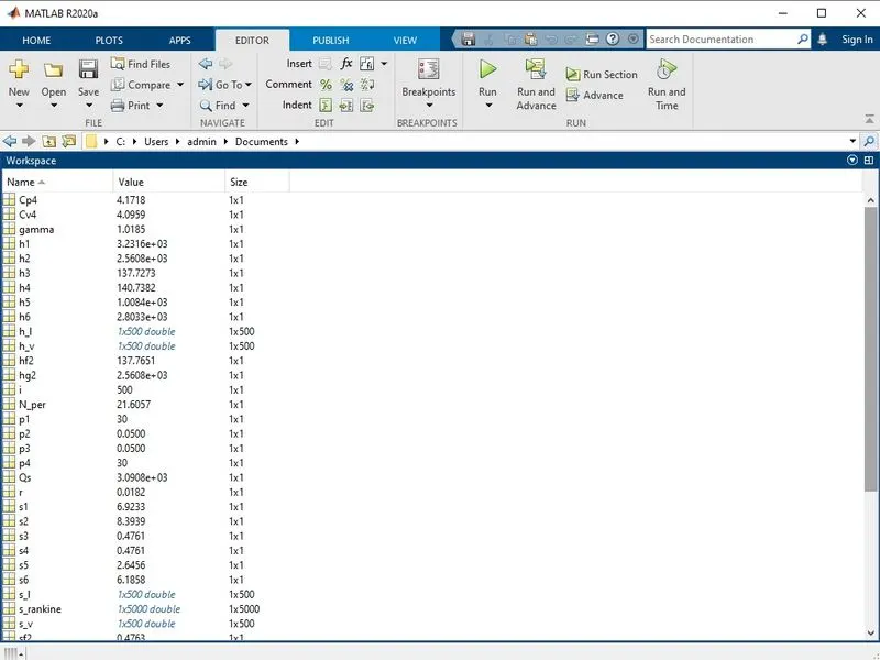
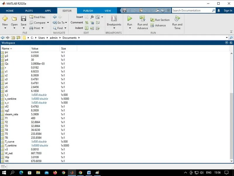
WORKSPACE:

PLOTS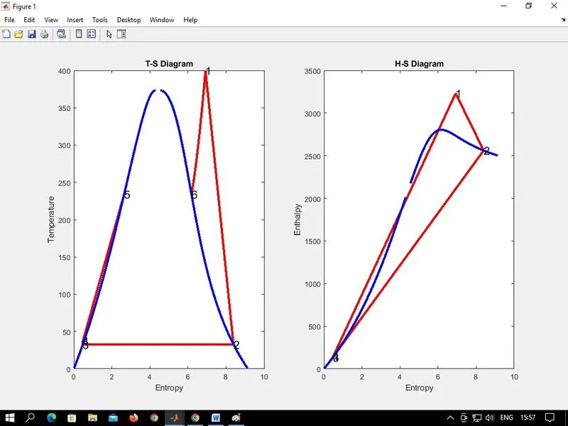

RESULT:

The rankine cycle plots have generated by calculating the state points, efficiency and the output is printed in the command window.