Curve Fitting
AIM: Write a program to fit linear and cubic polynomial for the specific heat(cp) data set and calculating goodness of fit using different parameters and different ways to improve the fit in MATLAB.
THEORY: Curve fitting is the process of constructing a curve, or mathematical function, that has the best fit to a series of data points, possibly subject to constraints. Curve fitting can involve either interpolation, where an exact fit to the data is required, or smoothing, in which a "smooth" function is constructed that approximately fits the data. A related topic is regression analysis, which focuses more on questions of statistical inference such as how much uncertainty is present in a curve that is fit to data observed with random errors. Fitted curves can be used as an aid for data visualization, to infer values of a function where no data are available, and to summarize the relationships among two or more variables. Extrapolation refers to the use of a fitted curve beyond the range of the observed data, and is subject to a degree of uncertainty since it may reflect the method used to construct the curve as much as it reflects the observed data.
Fitting lines and polynomial functions to data points
The first degree polynomial equation
Y = ax+b
is a line with slope a. A line will connect any two points, so a first degree polynomial equation is an exact fit through any two points with distinct x coordinates.
If the order of the equation is increased to a second degree polynomial, the following results:
Y = ax^2+bx+c
This will exactly fit a simple curve to three points.
If the order of the equation is increased to a third degree polynomial, the following is obtained:
Y = ax^3+bx^2+cx+d
This will exactly fit four points.
Goodness of Fit Statistics
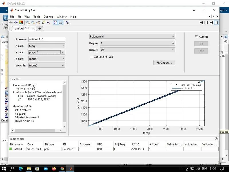
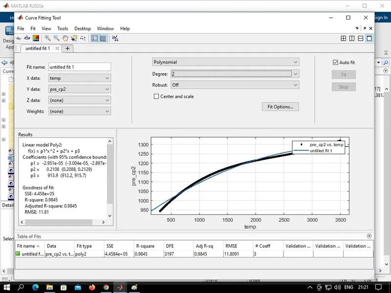
After using graphical methods to evaluate the goodness of fit, you should examine the goodness of fit statistics. The Curve Fitting Toolbox supports these goodness of fit statistics for parametric models:
- The sum of squares due to error (SSE)
- R-square
- Adjusted R-square
- Root mean squared error (RMSE)
- Sum of Squares Due to Error: This statistic measures the total deviation of the response values from the fit to the response values. It is also called the summed square of residuals and is usually labelled as SSE.
A value closer to 0 indicates a better fit. - R_square: R-square-This statistic measures how successful the fit is in explaining the variation of the data. It can also be under stood as the square the correlation between the response values and the predicted response values. It defined as the ratio of the sum of squares of the regression (SSR) and the total sum of squares (SST).
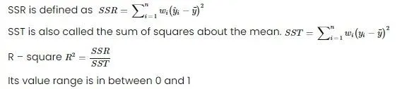
- Adjusted R-square: This statistic uses the R-square statistic defined above, and adjusts it based on the residual degrees of freedom. It is generally the best indicator of the quality when you compare two models that are nested that is, a series of models each of which adds additional coefficients to the previous model.

- Roof Mean Squared Error (RMSE): This statistic is also known as the standard error and te standard error of the regression. It is an estimate of the standard deviation of the random component in the data.

Using these four-quantities MATLAB effectively deduces the goodness of fit, typically R_square is greater than 0.95 the fit is assumed to be good.
PROCEDURE:
FOR LINEAR AND CUBIC FIT
- As MATLAB is a case sensitive software, make sure of that during the programming. And clear and close all the previous data before starting.
close all (closes all the previous plots )
clear all (clears all the variable data )
clc (clears the command window)
- Now load the data by “cp_data = load(‘data’)” make sure the data is in same loacation where the program is going to save. Now enter the inputs of temperature and specific heat(cp) as “temp = cp_data(:,1)” & “cp = cp_data(:,2)” as the 1st column is for temperature and 2nd is for specific heat.
- Now curve fit for 1 degree polynomial is created, "polyfit" command is used to calculate the values of the coefficients and then with “polyval" the values of "pre_cp1" is calculated with coefficients and the temperature. Now follow the same steps for 3 degree polynomial Now for curve fitting the data of 1 degree polynomial data. Open a new figure window using "figure" command, with "plot command plot the original data, and then plot the 1 degree polynomial data.
- Now for labelling the x-axis and y-axis use "xlabel and "ylabel" respectively. Now provide legends for differentiating the data by using legends command, for giving a title using "title" command. Follow the same steps for 3 degree polynomial data.
- Now for calculating SSE. SS SST, R_sq. R_sq_adj, RMSE. First for 1 degree polynomial and then for 3 degree polynomial. Calculate the error, then mean "M" using "mean command also provide with the number of independent variables "k". Now use the formulas for calculating different parameters that helps us determine the Goodness of fit.
CODE:
close all
clear all
clc

%inputs
cp_data = load('data'); %loads the data
temp = cp_data(:,1); %as 1st column is for temperature
cp = cp_data(:,2); %as 2nd column is for cp

%for linear fit
%cp = ax+b
coeffs1 = polyfit(temp,cp,1); %calculate the value of coefficients
pre_cp1 = polyval(coeffs1,temp); %calculate the value of cp based upon coefficients & temperature

%plotting linear fit
figure(1)
plot(temp,cp,'linewidth',3,'color','b')
hold on
plot(temp,pre_cp1,'linewidth',3,'color','r')
%labelling
xlabel('temperature [K]')
ylabel('specific heat [KJ/Kmol-K]')
axis([0 4000 850 1400])
title('1 degree polynomial')
legend('original data','curve fit')
hold off
grid on

%for cubic fit
%cp = ax^3+bx^2+cx+d
coeffs2 = polyfit(temp,cp,3);
pre_cp2 = polyval(coeffs2,temp);

%plotting linear fit
figure(2)
plot(temp,cp,'linewidth',3,'color','m')
hold on
plot(temp,pre_cp2,'linewidth',3,'color','g')
%labelling
xlabel('temperature [K]')
ylabel('specific heat [KJ/Kmol-K]')
axis([0 4000 850 1400])
title('3 degree polynomial')
legend('original data','curve fit')
hold off
grid on

%calculating the SSE,SSR,SST,R_sq,R_sq_adj,RMSE for 1 degree polynomial
error1 = pre_cp1 - cp;
n = length(cp); %np. of data
k = 1; %no. of independent variable
M = mean(cp); %mean
%calculating SSE1
sse1 = (error1).^2;
SSE1 = sum(sse1);
%calculating SSR1
ssr1 = (pre_cp1-M).^2;
SSR1 = sum(ssr1);
%calculating SST1
SST1 = SSE1+SSR1;
%calculating R_sq1
R_sq1 = SSR1/SST1;
%calculating R_sq_adj1
R_sq_adj1 = 1-[(1-R_sq1)*(n-1)/(n-k-1)];
%calculating RMSE1
RMSE1 = (SSE1/n)^0.5;

%calculating the SSE,SSR,SST,R_sq,R_sq_adj,RMSE for 3 degree polynomial
error2 = pre_cp2 - cp;
n = length(cp); %np. of data
k = 3; %no. of independent variable
M1 = mean(cp); %mean
%calculating SSE2
sse2 = (error2).^2;
SSE2 = sum(sse2);
%calculating SSR1
ssr2 = (pre_cp2-M1).^2;
SSR2 = sum(ssr2);
%calculating SST2
SST2 = SSE2+SSR2;
%calculating R_sq2
R_sq2 = SSR2/SST2;
%calculating R_sq_adj2
R_sq_adj2 = 1-[(1-R_sq2)*(n-1)/(n-k-1)];
%calculating RMSE2
RMSE2 = (SSE2/n)^0.5;
FOR IMPROVING FIR (SPLITWISE METHOD)
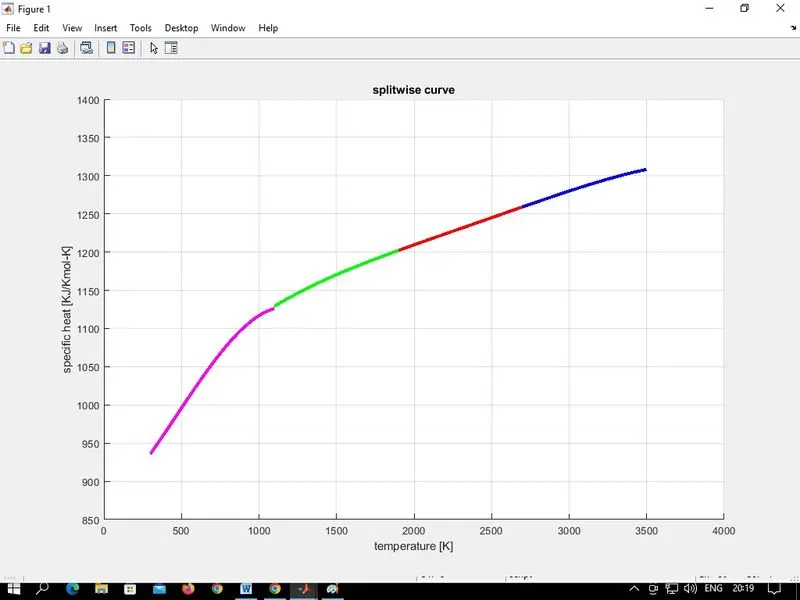
- The fit is divided into 4 parts so that it can fit properly, if needed it can be divided in more parts to get more precise result.
- Start with "clear", "close all", "clc” commands to clear the workspace, closing all the figures, and clear the command window.
- To start with the curve fit first data is loaded in a variable by using "load" command and Then the data of first column is assigned to a variable temperature and the second column contains the specific heat that is assigned to the variable "cp".
- Now divide the whole data into 4 parts that is 1-800, 800-1600, 1600-2400, and 2400- 3200. Now assign the values of temperature with suffix 1, 2, 3, 4) and cp (with suffix 1,2, 3, 4) in the variables.
- Now for curve fit use the "polyfit command for determining the coefficients of the polynomial and “polyval" command calculates the value of cp on the basis of coefficients and temperature. Here I have used a 5th degree polynomial and for that centering and scaling of "polyfit” command is used so that there are no warnings. Output of "polyfit” here is saved in three variables, as the degree of polynomial is therefore it requires four inputs for evaluating the new "cp".
- Now plot the data use the "plot" command, start with the original data, then using hold on command plot the date for the ranges 1-800, 801-1600, 1601-2400, and 2401 - 3200, Now for labeling the axis and y-axis use “xlabel" and "ylabel" respectively Now provide legends for differentiating the data by using "legends" command, for giving a title using "title" command.
CODE:
close all
clear all
clc

%curve fitting using splitwise method
%inputs
cp_data = load('data');
temp = cp_data(:,1);
cp = cp_data(:,2);

%diving the temperature & specific heat in 4 parts
temp1 = temp(1:800);
cp1 = cp(1:800);

temp2 = temp(800:1600);
cp2 = cp(800:1600);

temp3 = temp(1600:2400);
cp3 = cp(1600:2400);

temp4 = temp(2400:3200);
cp4 = cp(2400:3200);

%for linear fit
coeffs1 = polyfit(temp1,cp1,3);
pre_cp1 = polyval(coeffs1,temp1);

coeffs2 = polyfit(temp2,cp2,3);
pre_cp2 = polyval(coeffs2,temp2);

coeffs3 = polyfit(temp3,cp3,3);
pre_cp3 = polyval(coeffs3,temp3);

coeffs4 = polyfit(temp4,cp4,3);
pre_cp4 = polyval(coeffs4,temp4);

%plotting

hold on
plot(temp1,pre_cp1,'linewidth',3,'color','m')
plot(temp2,pre_cp2,'linewidth',3,'color','g')
plot(temp3,pre_cp3,'linewidth',3,'color','r')
plot(temp4,pre_cp4,'linewidth',3,'color','b')
xlabel('temperature [K]')
ylabel('specific heat [KJ/Kmol-K]')
axis([0 4000 850 1400])
title('splitwise curve')
hold off
grid on
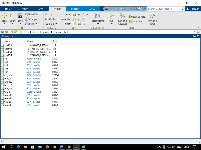
WORKSPACE AND GRAPHS:
FOR LINEAR AND CUBIC FIT
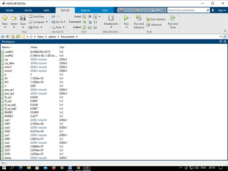
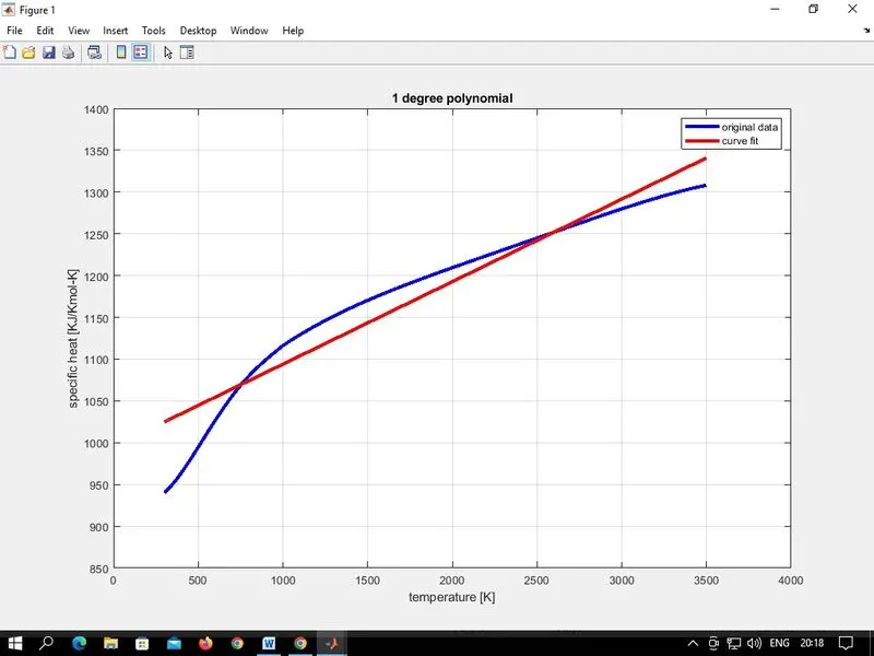
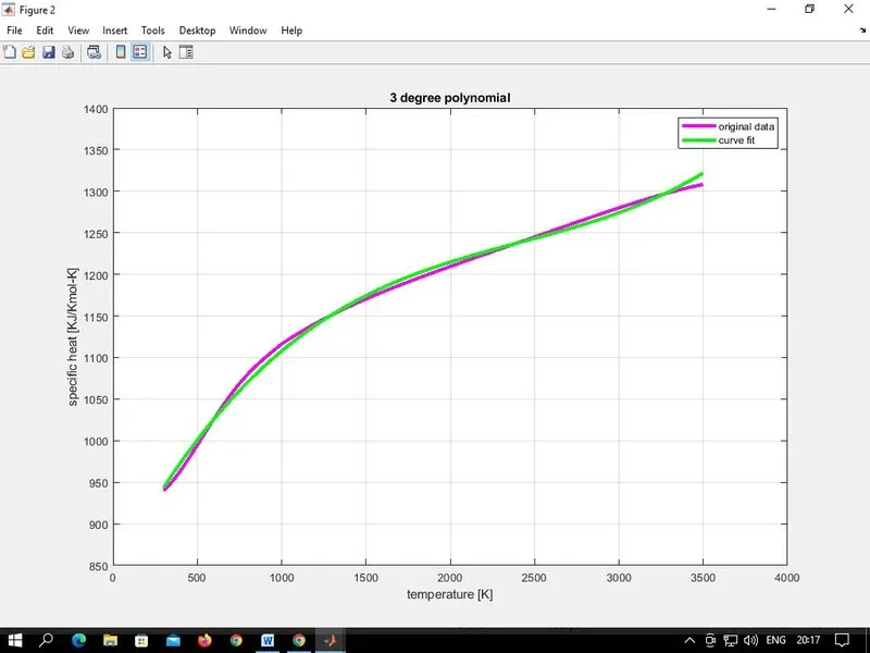
FOR SPLITWISE METHOD
USING TOOLBOX:
QUESTION AND ANSWER
Q. How make a curve fit perfectly?
A. Curve fit can be made perfect by interpolating the datasets. By interpolation, the errors can be minimized and it is also possible to reduce the errors to zero. Curve fit should match with the original data without showing the error in command window.
Q. How to get the best fit?
A: The best fit can be obtained by increasing the order of polynomial and also by splitting the curve fits into multiple numbers of polynomials for different sets of temperature and specific heat values. The best fit can also be chosen by our different ways:
Sum of Squares due to Error (SSE)
R-square
Adjusted R-square
Root Mean Squared Error (RMSE)
Q. What could be done to improve the curve fit?
A. The cubic fit can be improved by splicing the curve fits into multiple numbers polynomials for different sets of temperature values. It can also be improved by reducing the error between the original data set and curve fit value.
REFERENCES: