Week -3 Challenge
FOR UDDS
clear all
close all
clc
fprintf('WEEK-3 CHALLENGE FOR UDDS DATA')
%inputs
M = 2400; %vehicle weight
g = 9.81; %gravity
Cd = 0.35; %drag coeficient
Af = 2.4; %frontal area vehicle
rho = 1.225; %air density
Cr = 0.013; %rolling resistance
Aft = 5; %trailer frontal area
Cdt = 0.8; %trialer drag force
Tw = 1250; %trailer weight
%tire size
sw = 0.245; %section width
wd = 0.4572; %wheel diameter
hs = 60/100*sw;
Td = (2*hs)+wd; %tire diameter
Tr = Td/2; %tire radius
rr = 97/100*Tr; %rolling radius
%loading the file
% f1= load('udds.txt');
% time = f1(:,1);
% s = f1(:,2); %in mph
% speed = s/3600; %in mps

dc=xlsread("UDDS.xlsx");
time =dc(:,1);
speed =dc(:,2);

range = length(speed)-1;

for i = 1:range;
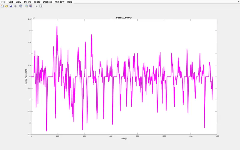
a(i) = speed(i+1)-speed(i); %acceleration
a_f(i) = M.*a(i); %acceleration force
a_p(i) = a_f(i).*speed(i); %acceleration power
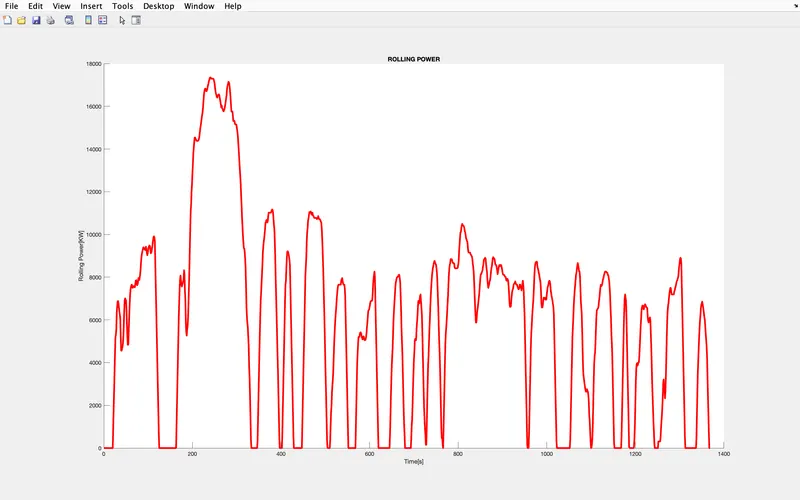
r_f(i) = Cr*M*g; %rolling force
r_p = r_f(i).*speed; %rolling power
aero_force(i) = 0.5*rho*Af*Cd*speed(i).^2;
aero_p(i) = aero_force(i).*speed(i);
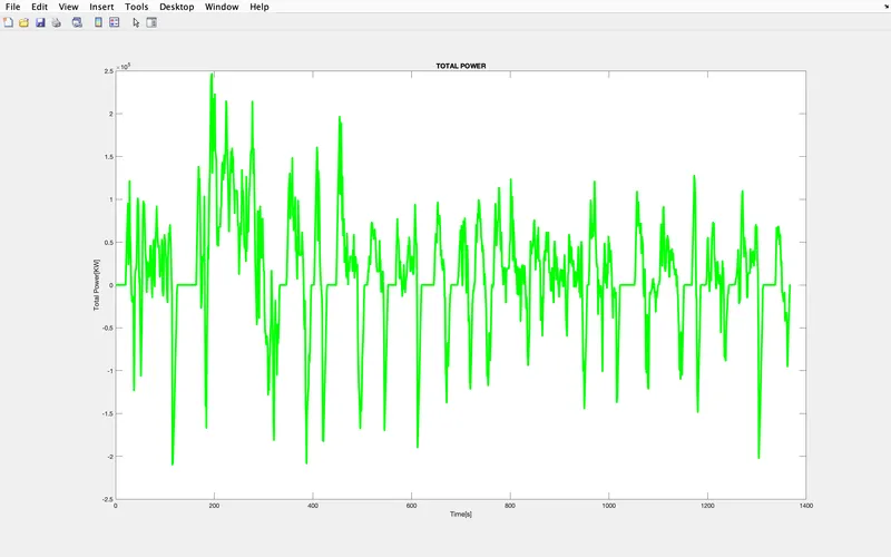
t_f(i) = a_f(i)+r_f(i)+aero_force(i); %total force
t_p(i) = t_f(i).*speed(i); %total power
end
%seperating positive and negative values of total power
n_nos = (t_p(t_p<0));
p_nos = (t_p(t_p>=0));
%engergy requirement
T = (time)';
t = time(1:1369);
e = t_p.*t; %energy
ep = e(e>0); %positive energy requirement
en = e(e<0); %negitive energy requirement
tpe = sum(ep); %sum of positive energy
tpn = sum(en); %sum of positive energy

avg_pnos = mean(p_nos);
max_pnos = max(p_nos);
max_nnos = max(n_nos);

%energy requirement with regen when power is limited to 10, 20, 30, 45, 60 kW and 80% efficient.

e_10 = sum(10.*t)*0.8;
e_lim_10 = tpe-e_10;
e_20 = sum(20.*t)*0.8;
e_lim_20 = tpe-e_20;
e_30 = sum(30.*t)*0.8;
e_lim_30 = tpe-e_30;
e_45 = sum(45.*t)*0.8;
e_lim_45 = tpe-e_45;
e_60 = sum(60.*t)*0.8;
e_lim_60 = tpe-e_60;
p_lim = [10 20 30 45 60];
e_reg = [e_lim_10 e_lim_20 e_lim_30 e_lim_45 e_lim_60];


%plotting
hold on
figure(1)
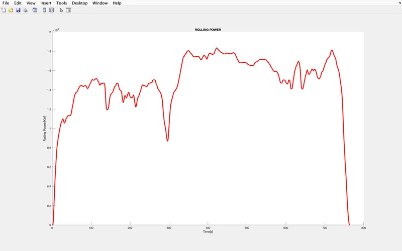
plot(time,r_p,'linewidth',3,'color','r');
title('ROLLING POWER')
xlabel('Time[s]')
ylabel('Rolling Power[KW]')
figure(2)
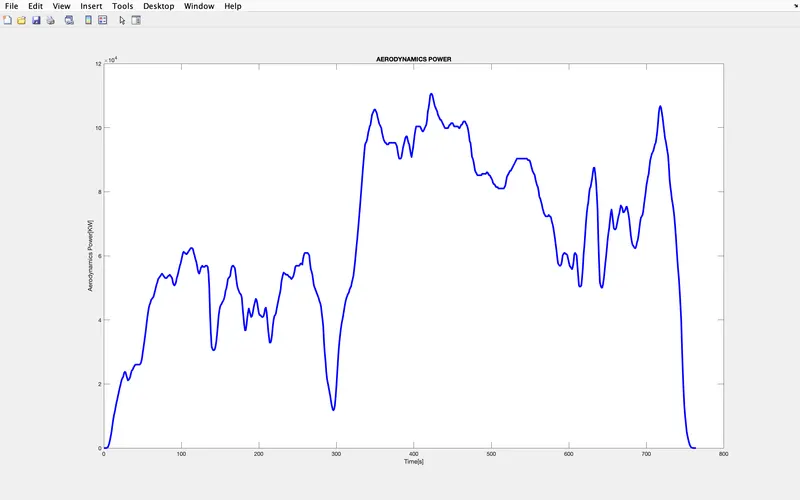
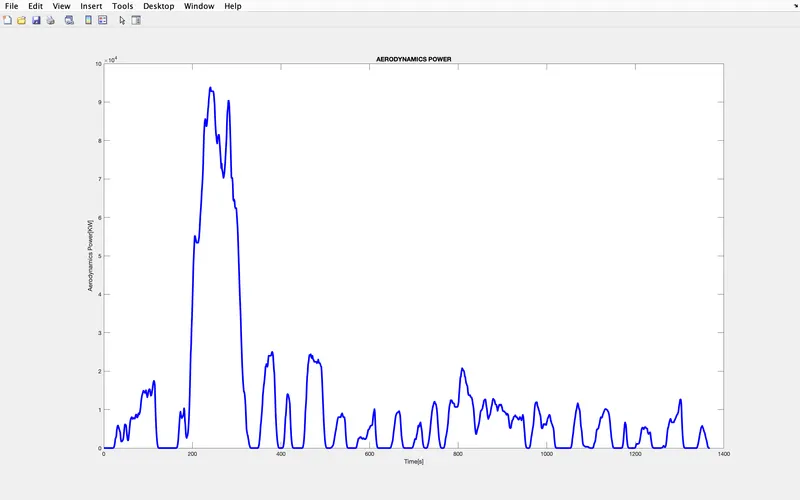
plot(t,aero_p,'linewidth',3,'color','b');
title('AERODYNAMICS POWER')
xlabel('Time[s]')
ylabel('Aerodynamics Power[KW]')
figure(3)
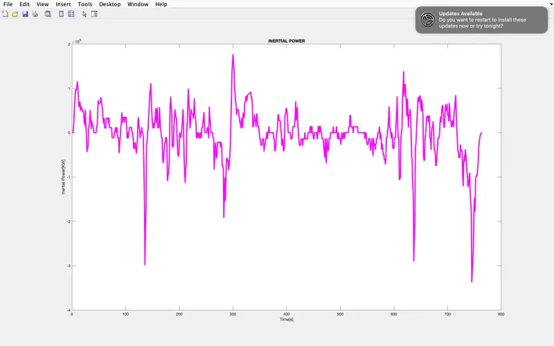
plot(t,a_p,'linewidth',3,'color','m');
title('INERTIAL POWER')
xlabel('Time[s]')
ylabel('Inertial Power[KW]')
figure(4)
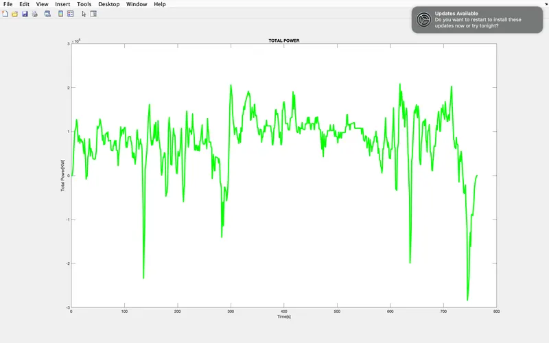
plot(t,t_p,'linewidth',3,'color','g');
title('TOTAL POWER')
xlabel('Time[s]')
ylabel('Total Power[KW]')
figure(5)
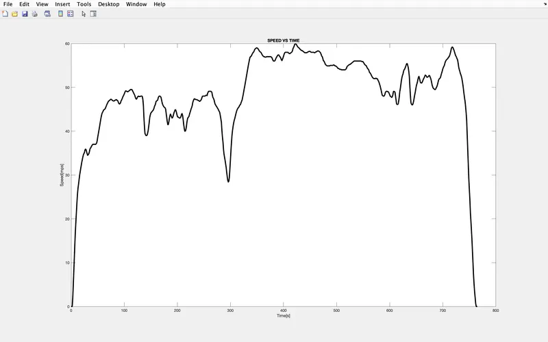
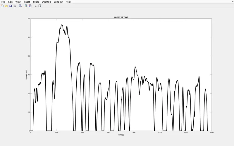
plot(time,speed,'linewidth',3,'color','k');
title('SPEED VS TIME')
xlabel('Time[s]')
ylabel('Speed[mps]')
figure(6)
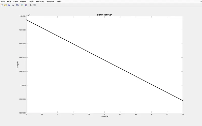
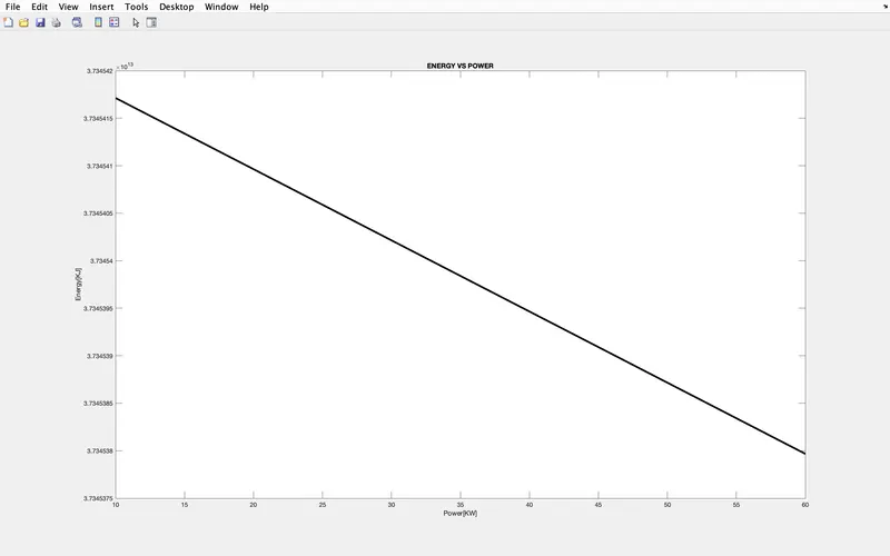
plot(p_lim,e_reg,'linewidth',3,'color','k');
title('ENERGY VS POWER')
xlabel('Power[KW]')
ylabel('Energy[KJ]')

hold off
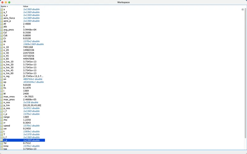
WORKSPACE
PLOTS
FOR HWFET
clear all
close all
clc
fprintf('WEEK-3 CHALLENGE FOR HWFET DATA')
%inputs
M = 2400; %vehicle weight
g = 9.81; %gravity
Cd = 0.35; %drag coeficient
Af = 2.4; %frontal area vehicle
rho = 1.225; %air density
Cr = 0.013; %rolling resistance
Aft = 5; %trailer frontal area
Cdt = 0.8; %trialer drag force
Tw = 1250; %trailer weight
%tire size
sw = 0.245; %section width
wd = 0.4572; %wheel diameter
hs = 60/100*sw;
Td = (2*hs)+wd; %tire diameter
Tr = Td/2; %tire radius
rr = 97/100*Tr; %rolling radius
%loading the file
% f1= load('udds.txt');
% time = f1(:,1);
% s = f1(:,2); %in mph
% speed = s/3600; %in mps

dc=xlsread("HWFET.xlsx");
time =dc(:,1);
speed =dc(:,2);

range = length(speed)-1;

for i = 1:range;
a(i) = speed(i+1)-speed(i); %acceleration
a_f(i) = M.*a(i); %acceleration force
a_p(i) = a_f(i).*speed(i); %acceleration power
r_f(i) = Cr*M*g; %rolling force
r_p = r_f(i).*speed; %rolling power
aero_force(i) = 0.5*rho*Af*Cd*speed(i).^2;
aero_p(i) = aero_force(i).*speed(i);
t_f(i) = a_f(i)+r_f(i)+aero_force(i); %total force
t_p(i) = t_f(i).*speed(i); %total power
end
%seperating positive and negative values of total power
n_nos = (t_p(t_p<0));
p_nos = (t_p(t_p>=0));
%engergy requirement
T = (time)';
t = time(1:765);
e = t_p.*t; %energy
ep = e(e>0); %positive energy requirement
en = e(e<0); %negitive energy requirement
tpe = sum(ep); %sum of positive energy
tpn = sum(en); %sum of positive energy

avg_pnos = mean(p_nos);
max_pnos = max(p_nos);
max_nnos = max(n_nos);

%energy requirement with regen when power is limited to 10, 20, 30, 45, 60 kW and 80% efficient.

e_10 = sum(10.*t)*0.8;
e_lim_10 = tpe-e_10;
e_20 = sum(20.*t)*0.8;
e_lim_20 = tpe-e_20;
e_30 = sum(30.*t)*0.8;
e_lim_30 = tpe-e_30;
e_45 = sum(45.*t)*0.8;
e_lim_45 = tpe-e_45;
e_60 = sum(60.*t)*0.8;
e_lim_60 = tpe-e_60;
p_lim = [10 20 30 45 60];
e_reg = [e_lim_10 e_lim_20 e_lim_30 e_lim_45 e_lim_60];


%plotting
hold on
figure(1)
plot(time,r_p,'linewidth',3,'color','r');
title('ROLLING POWER')
xlabel('Time[s]')
ylabel('Rolling Power[KW]')
figure(2)
plot(t,aero_p,'linewidth',3,'color','b');
title('AERODYNAMICS POWER')
xlabel('Time[s]')
ylabel('Aerodynamics Power[KW]')
figure(3)
plot(t,a_p,'linewidth',3,'color','m');
title('INERTIAL POWER')
xlabel('Time[s]')
ylabel('Inertial Power[KW]')
figure(4)
plot(t,t_p,'linewidth',3,'color','g');
title('TOTAL POWER')
xlabel('Time[s]')
ylabel('Total Power[KW]')
figure(5)
plot(time,speed,'linewidth',3,'color','k');
title('SPEED VS TIME')
xlabel('Time[s]')
ylabel('Speed[mps]')
figure(6)
plot(p_lim,e_reg,'linewidth',3,'color','k');
title('ENERGY VS POWER')
xlabel('Power[KW]')
ylabel('Energy[KJ]')

hold off
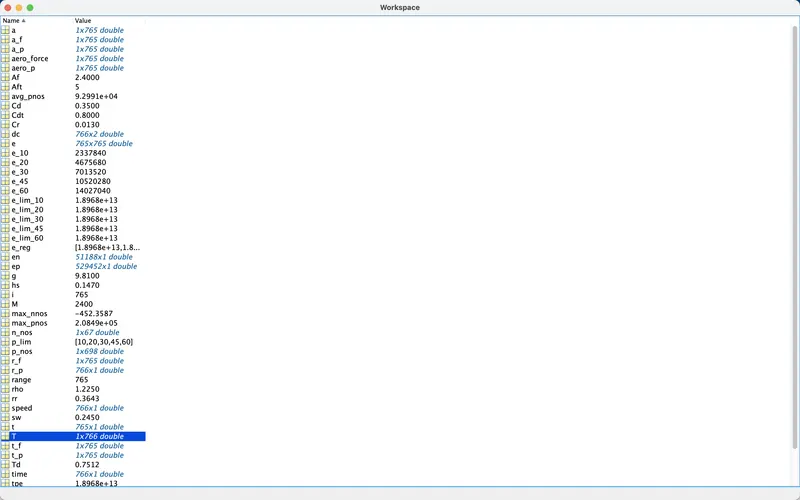
WORKSPACE
PLOTS