solving the ODE

AIM: Write a program in Matlab to solve the ODE and to simulate the motion of pendulum with damping.

THEORY: In mathematics, an ordinary differential equation (ODE) is a differential equation containing one or more functions of one independent variable and the derivatives of those functions. The term ordinary is used in contrast with the term partial differential equation which may be with respect to more than one independent variable.

For a sile pendulum with a damping factor the equation for simple pendulum is:

Where,

• b = damping coefficient (N-m/s)
• m = mass of the bob (kg)
• g = gravitational acceleration (m/s)
• l = length of the string to connect bob (m)

PROCEDURE:

FOR THE MAIN PROGRAM

• As MATLAB is a case sensitive software, make sure of that during the programming. And clear and close all the previous data before starting.

close all (closes all the previous plots )

clear all (clears all the variable data )

clc (clears the command window)

• Now enter the input values such as damping coefficient, gravitational pull, length of string & mass of the bob.
• Now define the initial condition of angular displacement and angular velocity in a variable theta_0.
• Now define the time span value with the variable t_span. Use linspace command to give the value from ‘0’ to ‘20’ having ‘250’ values with equal interval.

ODE SOLVER

• In MATLAB there is a in-built solver which is ‘ODE45’ to solve the differential equation. The syntax of ‘ode45’ is first we define the independent and dependent variable ‘@(t,theta)’ then the function is called that contains the ode function i.e. “ode_function(t,theta,b,g,l,m) then the time span is given for which function is integrated ‘t_span’ and then the initial condition is given ‘theta_0’. All results are stored in a array [t,results].

PLOTTING

• Now using the plot command, plot the graph between the time and the results(angular displacement & angular velocity). First select the data of all rows and first column (:,1) and then us the hold on command and plot the second graph having the all rows and second column.
• Now use some line styling command like linewidth, color.
• Now label the x-axis and y-axis as time and plot and use the legend command and name the lines as angular displacement and angular velocity. Set the axis([0 20 -5 5]) andfor a better view on the grid “grid on”.

ANIMATION

• Now for creating the animation ‘for’ loop is used. Take i =1:length (results(:,1)) and then the enter the coordinates as x0 = 0, y0 = 0 , x1 = l*sin(results(i,1) &y1 = - l*cos(results(i,1).
• Now for plotting the values of x and y we use plot command. The command used for differentiating the two links is ‘legend’ which helps us to determine the links with color. The label the axis with command ‘xlabel’ & ‘ylabel’. A pause command is used for pausing the program for a certain time before processing a new set of values.
• Now for creating a video or a animation of the result a counter variable is defined before the first for loop command as ‘ct’ and then a variable ‘M’ for capturing the current frame every time ‘for’ command runs. For every increment of the frame ‘1’ is added to the variable ‘ct’. now close the loop command with ‘end’.
• Now for creating a movie command is used “movie(M) and for assigning the path and name of file ‘VideoWriter’ is used and is saved in ‘.avi’ format. For opening and closing the video “open” & “close” command is used. For writing the video with plot frames ‘writeVideo’ command is used.
• Run or compile the program with ‘F5’. The video will saved where the code is being saved.

FOR FUNCTION PROGRAM

• For function the name of the function should be same with the name of the file as ode_function.
• Now break the 2^ND order ODE into two first order ODE as ‘dtheta1_dt’ and ‘dtheta2_dt’.
• Now the two results is combined in an array ‘dtheta_dt’ which contains the value in two rows.

CODE:

FOR MAIN PROGRAM:

close all
clear all
clc

%inputs
b = 0.05; %Damping coefficient(Nm/s)
g = 9.81; %Gravity (m/s)
l = 1.5; %Length of string (m)
m = 0.1; %Mass of the ball (kg)

%intial condiion
theta_0 = [0;3]; %Initial condition of angular displacement & velocity
%time points
t_span = linspace(0,20,500);
%solve ode
[t,results] = ode45(@(t,theta)ode_function(t,theta,b,g,l,m),t_span,theta_0);

%plotting
figure(1)
plot(t,results(:,1),'linewidth',3,'color','r');
hold on
plot(t,results(:,2),'linewidth',3,'color','b');
xlabel('time');
ylabel('plot');
legend('angular displacement','angular velocity');
axis([0 20 -5 5])
hold off
grid on

%animation
RESULT = results(:,1);
ct = 1;
for i = 1:length(RESULT);
    A = RESULT(i);
    x0 = 0;
    y0 = 0;
    x1 = l*sind(A);
    y1 = -l*cosd(A);
    
    figure(2)
    plot([-1 1],[0 0],'linewidth',2,'color','g');
    hold on
    line([x0 x1],[y0 y1],'linewidth',2,'color','k');
   plot(x1,y1,'marker','o','markersize',20,'markerfacecolor','r');
   axis([-1.5 1.5 -2 2]);
   hold off
    pause(0.03);
    M(ct) = getframe(gcf);
    ct = ct+1;
end

movie(M) %creates a movie
videofile = VideoWriter('Ode_challenge.avi','uncompressed AVI') %assign the file name & format
open(videofile) %open the video
writeVideo(videofile,M) %write the video with plot frame
close(videofile) %closes the video

FOR FUNCTION:

function [dtheta_dt] = ode_function(t,theta,b,g,l,m)
theta1 = theta(1);
theta2 = theta(2);
dtheta1_dt = theta2;
dtheta2_dt = -(b/m)*theta2 -(g/l)*sind(theta1);
dtheta_dt = [dtheta1_dt; dtheta2_dt];
end

RESULT:

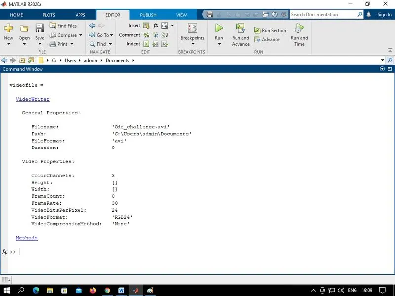
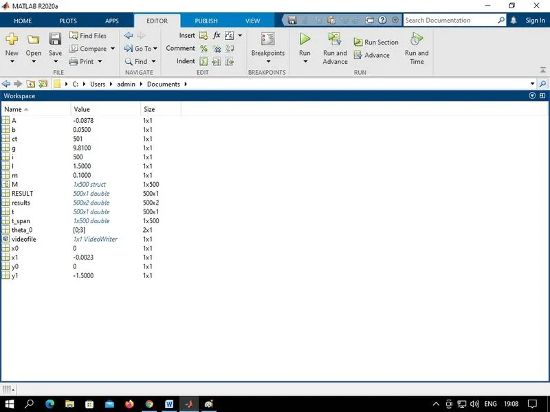
WORKSPACE:

ANIMINATION: https://youtu.be/ODDFPlT6gLQ

CONCLUSION:

The the motion of pendulum with damping is stimulated.