Week 8- Moving zones approach in Fluent

AIM:

• To simulate rotary motion for the given geometry and to study the moving zones approach in Fluent.

THEORY:

1: Introduction to moving zone:

• Two types of motion are involved in the fluid flow problem
  1. Rectilinear
  2. Rotary
• To model rotary motion, two approaches are used

1. Moving Reference Frame (MRF)
2. Moving Mesh Method (MMM)

Moving Reference Frame (MRF): it describes the use of a single moving reference frame, multiple moving reference frames, and mixing planes in Ansys Fluent. MRF approach is a steady-state method employed in industrial computational fluid dynamics to model problems with rotating parts.

• Single reference frame: Refer the entire computational domain to a single moving reference frame approach.
• Multiple reference frame: In complex geometry, it is not possible to use a single reference frame. In such cases break up the problem into multiple cell zones with well-defined interfaces between the cell zones.
  In Ansys Fluent, by enabling the moving reference frame in selected cell zones, we can model the problem involving moving parts. when the moving reference frame is activated, equations of motion are modified by incorporating the additional acceleration term due to the transformation stationary reference frame to a moving reference frame. By solving these equations in a steady state manner, the flow around the moving parts can be modelled.

Circular interface:

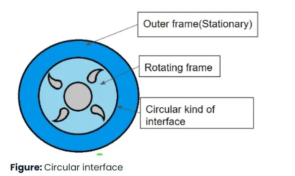
• The Navier-stoke equation in a stationary frame is solved separately
• Navier-stoke equation in moving frame is solved separately
• data is transferred from one frame to another frame through the interface by using the following methods
• Area averaging
• Mass averaging
• Mixed-out approach (best method because of no averaging)
  • Solve the following equations
    1. X-Momentum
    2. Y-Momentum
    3. Z-Momentum
    4. Energy

2: Moving Mesh Method (MMM): It describes the sliding and deforming mesh in Ansys Fluent. MMM are adaptive techniques for solving partial differential equations where the grid involves to improve the approximation to the solution.

• Sliding mesh method: If unsteady interaction between stationary and moving parts is important then employ the sliding mesh method to capture the transient behaviour of the fluid flow.

S.No.	Moving Reference Frame (MRF)	Moving Mesh Method (MMM)
1.	Frame is moving	Mesh is moving
2.	Steady phenomenon if unsteadiness is not important	Unsteady phenomenon if unsteadiness is important
3.	No change in the control volume	Control volume changes with time
4.	Mesh topology remains the same	Topology changes with time

SETUP AND SOLUTION:

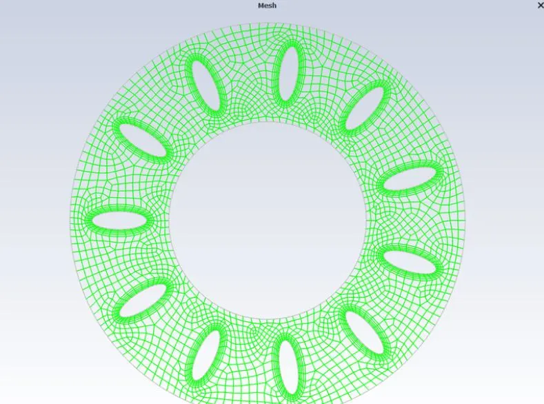
• First, we directly import the mesh file of the model into the solution set-up,
  
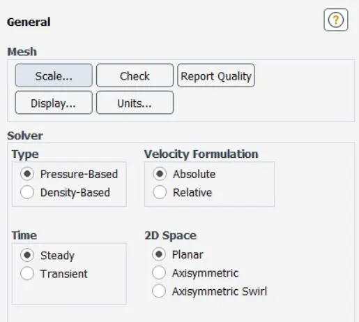
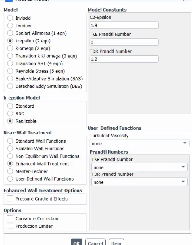
• Define it as a pressure-based solver. We choose the k-εε realizable model with enhanced wall treatment.

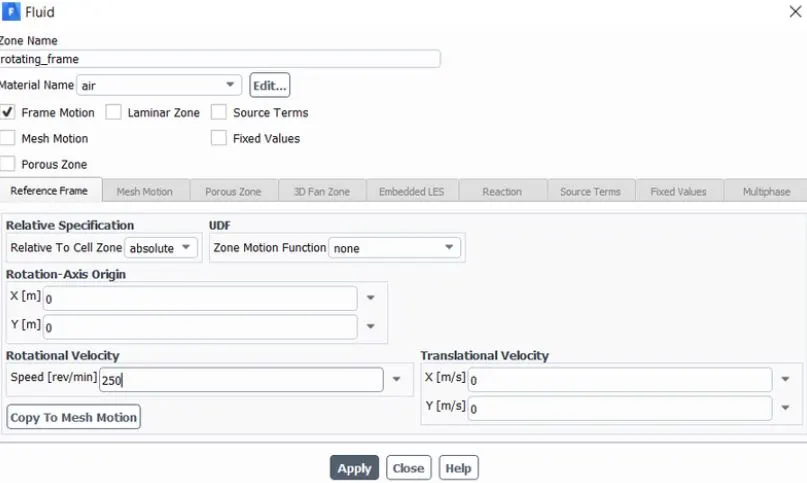
• Under cell zone conditions we set it to frame motion and give the rotational velocity as 250 rpm. The centre of rotation is given the default (0,0)

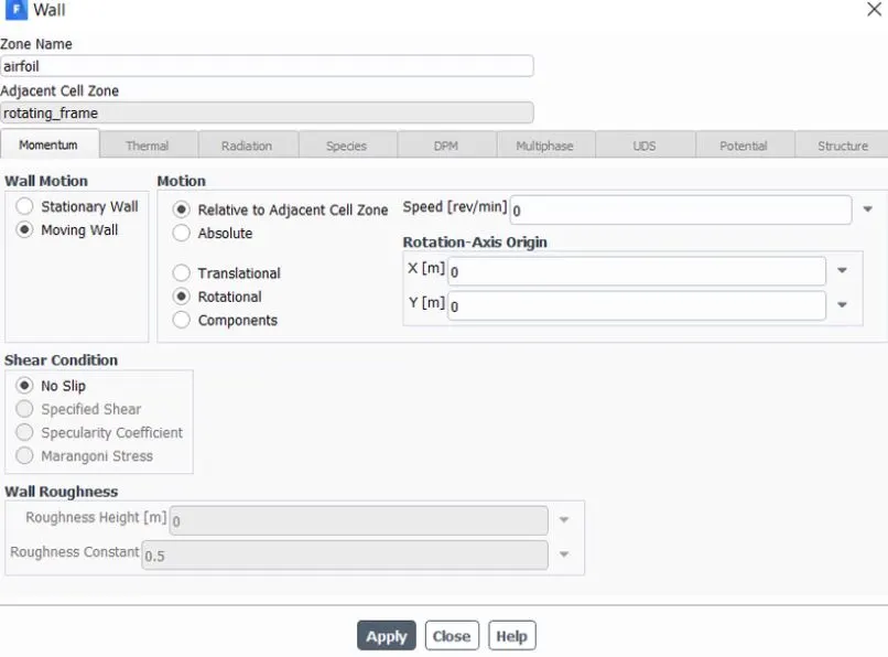
• Under boundary conditions for the airfoil, we check the relative to adjacent cell zone and Rotational motion.

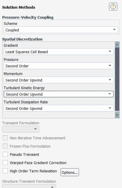
• In the solution methods, the scheme is set to coupled and the spatial discretization is set to second order upwind.

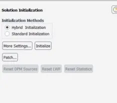
• Here the are no inlet and outlet conditions so we are doing hybrid initialization.

RESULT:

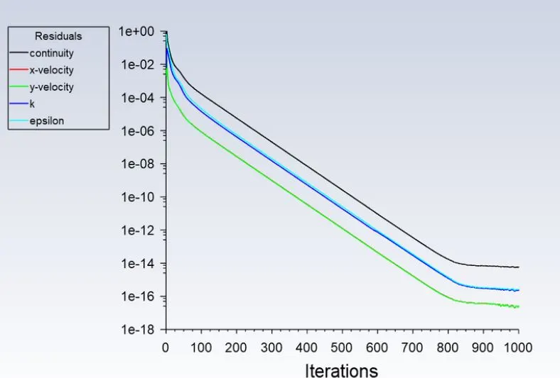
• RESIDUAL:

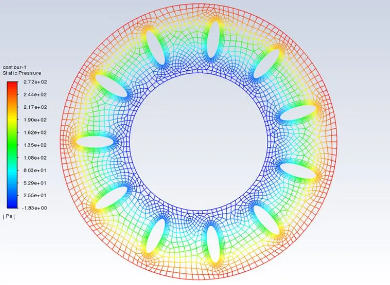
• PRESSURE:

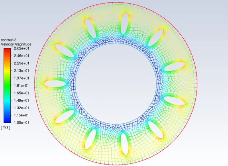
• VELOCITY:

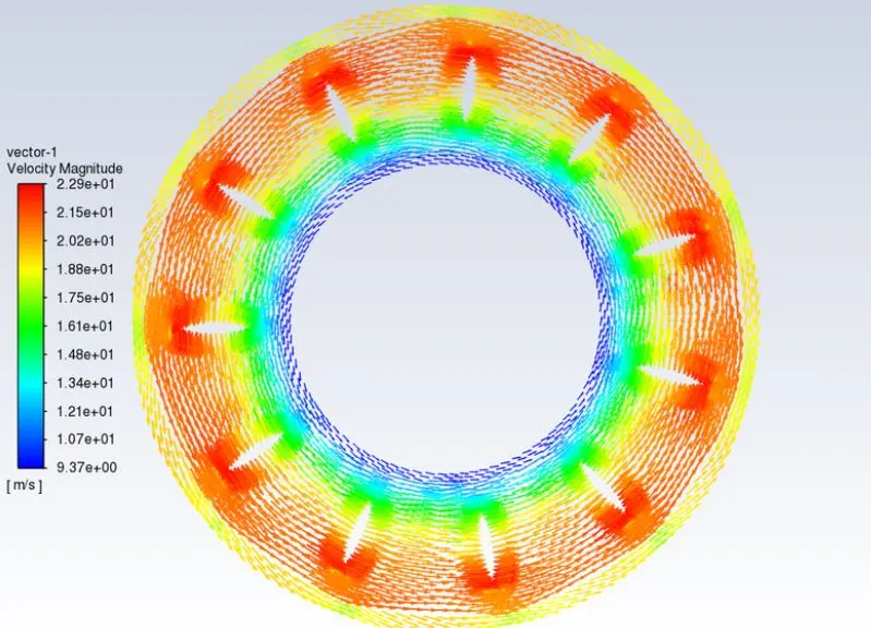
• VECTOR VELOCITY:

CONCLUSION:

• The maximum velocity (26 m/s) is at rotating domain_outer and the minimum velocity (10 m/s) is at rotating domain_inner.
• The largest velocity was observed in the outside frame in velocity contour plots, whereas the lowest velocity was recorded near the inner frame. However, by observing the airfoil edges, the top edge has been exposed to the most velocity, while the lower edge has been exposed to the lowest velocity. On top of the airfoil, the velocity separation can also be seen.
• Because the suction of air takes place near the centre of the impeller, the static pressure contour plot shows a low-pressure zone there. The velocity rises as it approaches the trailing edge of the airfoil until it reaches the impeller's maximum diameter.