Week 6 - CHT Analysis on a Graphics card

CHT Analysis on Graphics card

Aim

Perform a steady-state conjugate heat transfer analysis on a model of a graphics card.

Objective

1. Run the simulation by varying the velocity from 1m/sec to 5m/sec for at least 3 velocities and discuss the results.
2. Find out the maximum temperature and heat transfer coefficient attained by the processor.
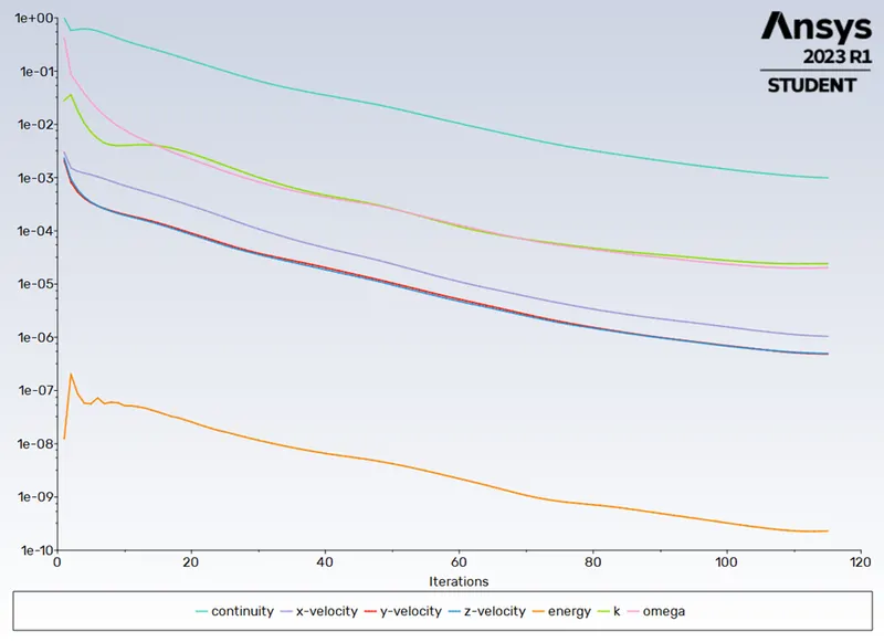
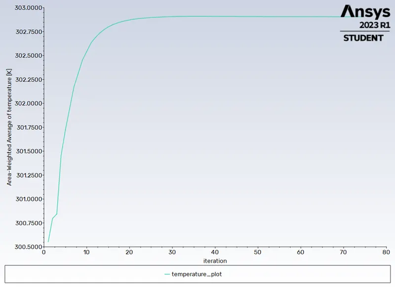
3. Prove that the simulation has achieved convergence with appropriate images and plots.
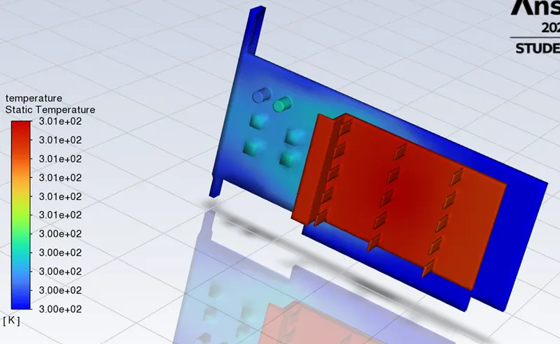
4. Identify potential hotspots on the model.

Conjugate Heat Transfer Analysis

Conjugate heat transfer analysis refers to a computational modelling technique used to analyse the combined effects of heat transfer through both solid materials and fluid mediums. It considers the interaction between fluid flow and heat transfer within a system, where heat is exchanged between the solid surfaces and the surrounding fluid.

In many engineering applications, such as electronics cooling, combustion systems, and thermal management in various industries, understanding the coupled behaviour of fluid flow and heat transfer is crucial for designing efficient and reliable systems.

Conjugate heat transfer analysis takes into account the thermal conduction within solid structures and convective heat transfer in the fluid. It considers the temperature distribution in both the solid and fluid domains, taking into consideration the interface between them.

To perform a conjugate heat transfer analysis, computational fluid dynamics (CFD) and computational heat transfer (CHT) methods are typically employed. These methods solve the governing equations for fluid flow and heat transfer simultaneously, coupling the fluid flow equations with the energy equations for both the solid and fluid domains.

Geometry

Graphics Card

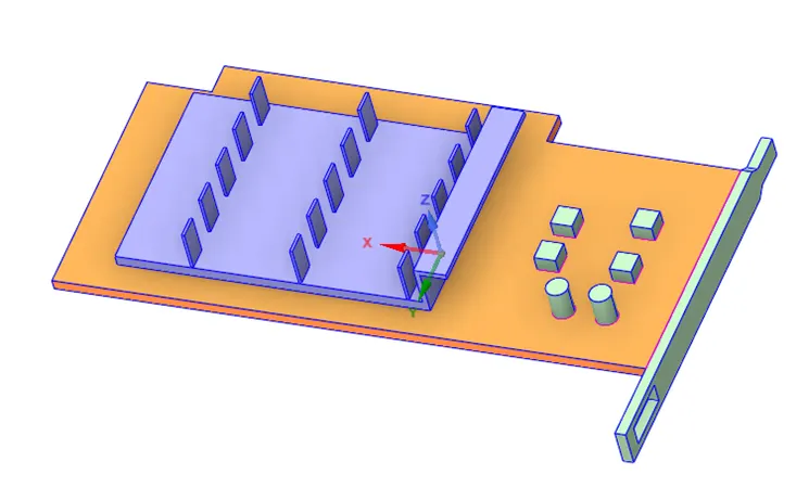
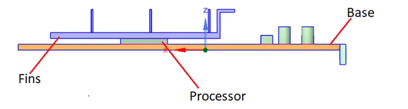
Enclosure

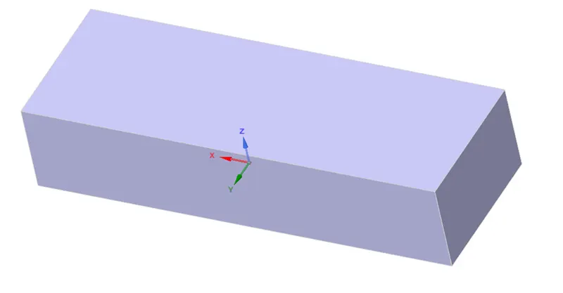
Share Topology enabled to avoid overlapping and non-conformal meshes

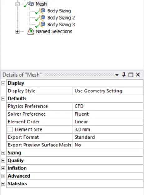
Mesh

Element Order : Linear

Element Size: 3 mm

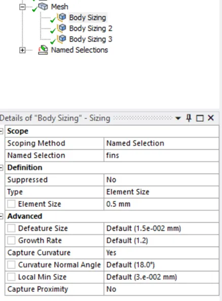
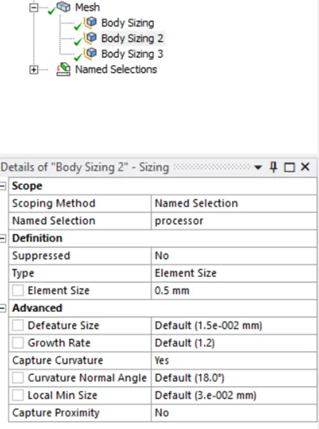
Body Sizing :

Fins & Processor

Element Size : 0.5 mm

Growth Rate : default (1.2)

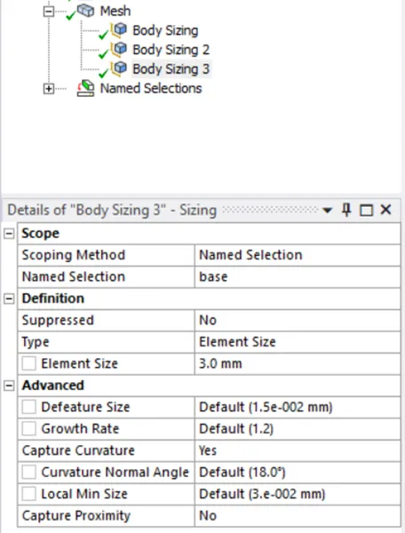
Body Sizing:

Base

Element Size : 3 mm

Growth Rate : default (1.2)

Setup

General:

Pressure-Based, Absolute, Steady-state

Model:

Energy

Viscous Model:

K-omega, SST

Material:

Solid

Fins: Aluminum

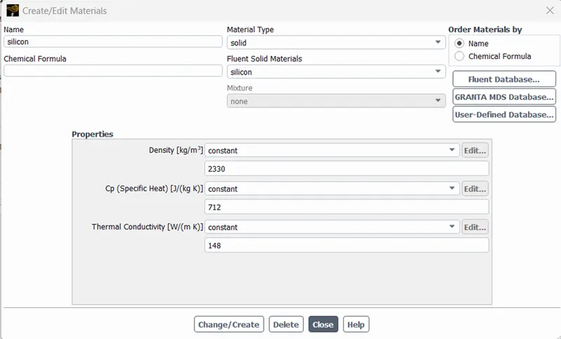
Processor: Silicon

Base : Wood

Fluid

Enclosure filled with Air

Silicon

Cell zones

Processor

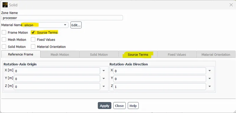
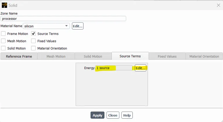
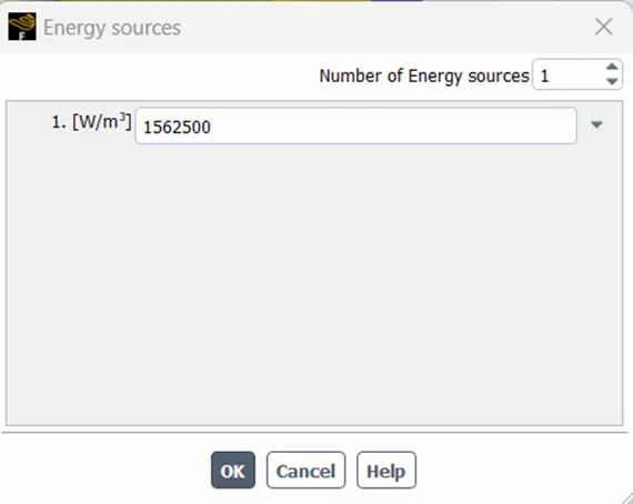
Heat Generated = Power / Volume

= 100 W / (8 x 8 x 1) mm³

= 1562500 W/m³

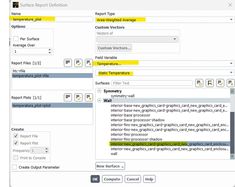
Report definition

Heat Transfer coefficient

Temperature

Result

Case 1: Velocity 5m/s

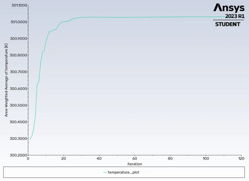
Temperature at the Processor = 301.03072 K

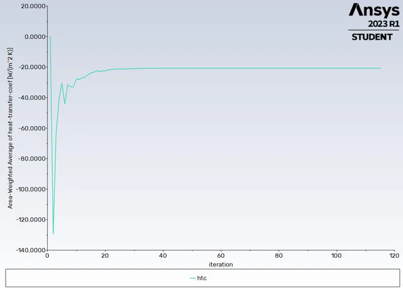
Heat Transfer Coefficient attained by the processor = 20 W/m². K

Scaled Residual

Temperature Plot

Heat Transfer Coefficient

Contours of static Temperature

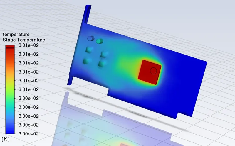
Case 2: Velocity = 3 m/s

Maximum Temperature attained by the processor = 301.40973 K

Heat transfer coefficient attained by the processor = 13.593545 W/m² .K

Scaled Residual

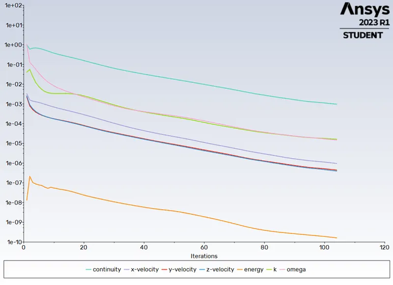
Temperature Plot

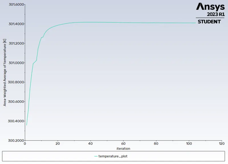
Heat Transfer Coefficient

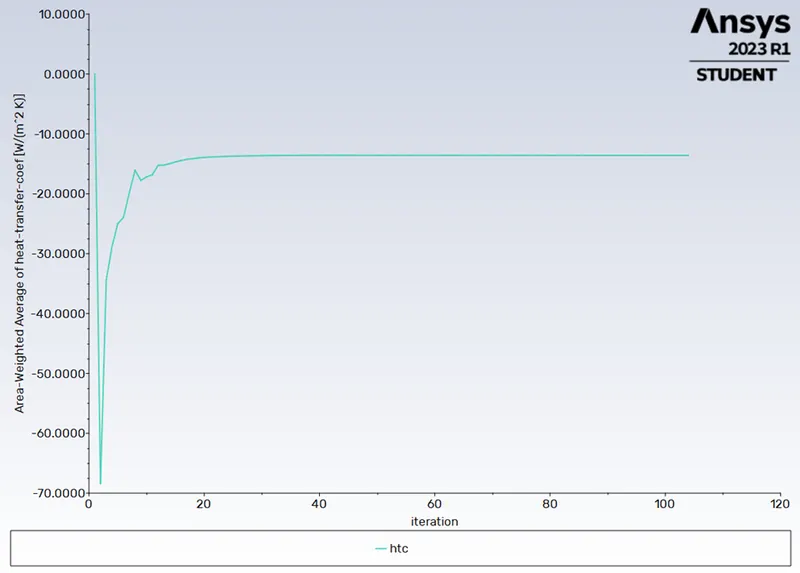
Temperature contour

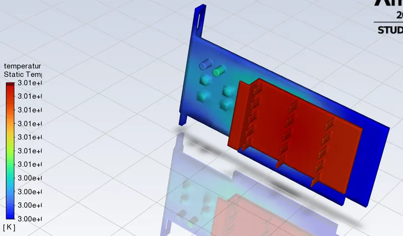
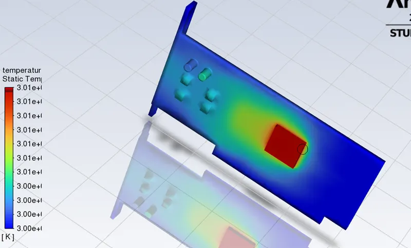
Case 3: Velocity = 1 m/s

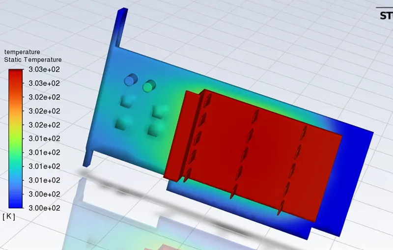
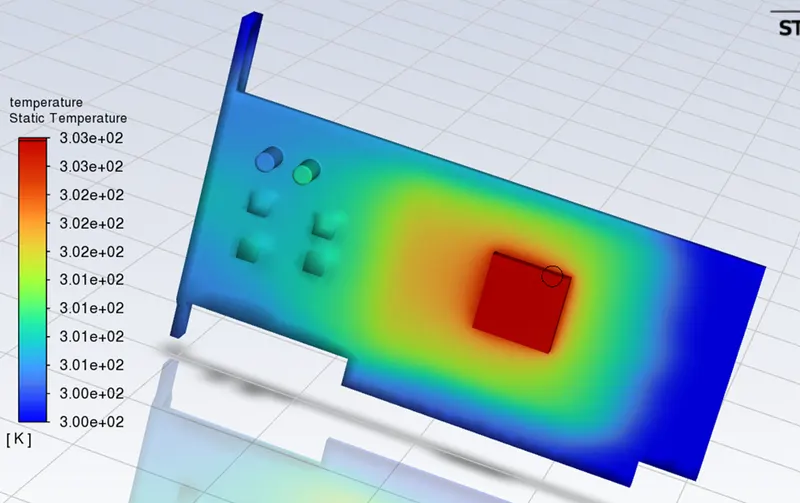
Maximum Temperature attained by the processor = 302.90513 K

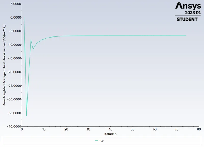
Heat transfer coefficient attained by the processor = 6.7536694 W/m² .K

Scaled Residuals

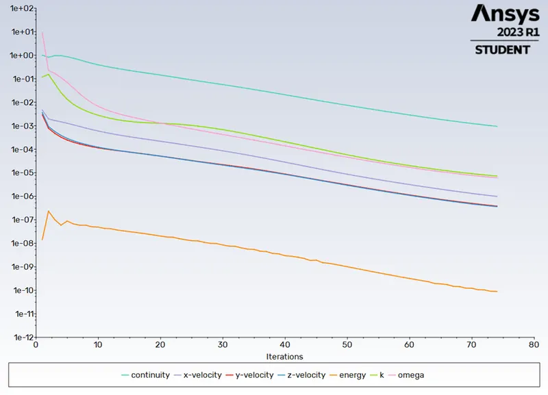
Temperature Plot

Heat Transfer Coefficient

Temperature Contour

Maximum Temperature and Heat Transfer Coefficient attained by the Processor

Velocity	Temperature (K)	Heat Transfer Coefficient (W/m2. K)
5 m/s	301.03	20
3 m/s	301.4	13.59
1 m/s	302.9	6.75

Analysing the above result, When Velocity is decreasing the Temperature attained by the Processor is increasing and the Heat Transfer Coefficient is decreasing. So the inlet Velocity is directly proportional to the Heat transfer Coefficient and indirectly proportional to the Temperature attained by the Processor.

Conclusion

Simulation of CHT Analysis on Graphics Card is performed for various inlet Velocity and the required plots are obtained to calculate the Temperature and Heat Transfer Coefficient.