Week 5 - Rayleigh Taylor Instability

Rayleigh Taylor Instability

Aim:

Simulation of Rayleigh Taylor instability waves using Ansys Fluent.

Objective:

1. What are some practical CFD models that have been based on the mathematical analysis of Rayleigh Taylor waves? In your own words, explain how these mathematical models have been adapted for CFD calculations.
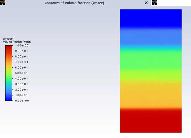
2. Perform the Rayleigh Taylor instability simulation for 2 different mesh sizes with the base mesh being 0.5 mm. Compare the results by showing the animations( Attach them from your google drive). Observe the differences in the animation and explain the effect of mesh size on simulation. Also, explain why a steady-state approach might not be suitable for these types of simulation.[ Choose Air and Water for this simulation]
3. Run one more simulation with water and user-defined material(density = 400 kg/m3, viscosity = 0.001 kg/m-s) for refined mesh.
4. Define the Atwood Number. Find out the Atwood number for both the cases and explain how the variation in Atwood number in the above two cases affects the behavior of the instability.

Rayleigh Taylor waves:

Rayleigh-Taylor (RT) waves are a type of fluid instability that occurs at the interface between two fluids of different densities when subjected to the influence of gravity. The phenomenon is named after Lord Rayleigh and G. I. Taylor, who extensively studied and described the behavior of these waves.

In an RT wave scenario, the denser fluid is typically located above the lighter fluid due to the force of gravity. However, if some perturbation or disturbance is introduced at the interface, it can lead to the development of complex wave-like patterns and mixing between the two fluids. The perturbation can arise from various sources, such as initial velocity differences, pressure variations, or surface roughness.

As the interface between the fluids becomes distorted, it results in the generation of upward- or downward-propagating waves, depending on the relative densities of the fluids. The denser fluid can penetrate into the lighter fluid, forming "fingers" or "spikes" that grow over time. Simultaneously, the lighter fluid can rise and form "bubbles" or "plumes" that displace the denser fluid above.

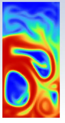
The growth of these waves is driven by the buoyancy force, which arises due to the density difference between the two fluids. The denser fluid, being heavier, is accelerated downwards by gravity, while the lighter fluid is accelerated upwards. This buoyant acceleration amplifies the initial perturbation, leading to the development of complex and intricate patterns.

Practical CFD models that have been based on the mathematical analysis of Rayleigh Taylor waves

One commonly used mathematical model for RT waves in CFD is based on the Navier-Stokes equations, which describe fluid flow and conservation of momentum. To adapt these equations for RT wave simulations, additional terms are introduced to account for the interfacial dynamics and buoyancy effects.

In RT wave CFD models, the governing equations are discretized in space and time to obtain a numerical approximation. Various numerical techniques, such as finite difference, finite volume, or finite element methods, can be employed for this purpose. These discretized equations are then solved iteratively using computational algorithms.

To model the interfacial dynamics, the interface between the two fluids is often tracked using methods like level set or volume-of-fluid (VOF). These methods represent the interface as a mathematical surface or a scalar field, respectively. The evolution of the interface is determined by solving advection equations for these quantities, considering the velocity and pressure fields obtained from the Navier-Stokes equations.

In addition to the interfacial dynamics, buoyancy effects play a crucial role in RT wave simulations. The buoyancy term is included in the Navier-Stokes equations to account for the acceleration due to the density difference between the fluids. This term is often modeled using the Boussinesq approximation, which assumes a linear relationship between density and temperature variations.

CFD models for RT waves also incorporate other physical phenomena, such as turbulence, heat transfer, and phase changes. Turbulence models, such as Reynolds-averaged Navier-Stokes (RANS) or large-eddy simulation (LES), are employed to capture the turbulent behavior at small scales. Heat transfer between the fluids can be modeled using energy conservation equations, considering conduction, convection, and phase change effects.

By simulating the behavior of RT waves using CFD models, researchers and engineers can gain insights into a wide range of practical applications. These models have been used to study phenomena such as supernova explosions, inertial confinement fusion, mixing processes in fluids, and various multiphase flow systems. The mathematical analysis of RT waves, adapted for CFD calculations, enables the investigation and prediction of complex fluid dynamics scenarios, aiding in design optimization, safety assessments, and scientific understanding.

Steady-state approach might not be suitable for the analysis of Rayleigh Taylor waves

A steady-state approach, where the flow variables remain constant with time, may not be suitable for simulating Rayleigh-Taylor (RT) waves due to the inherently unsteady and dynamic nature of this phenomenon. There are several reasons why a steady-state approach is inadequate for RT wave simulations:

1. Unstable and evolving interface: Rayleigh-Taylor waves involve the growth and evolution of the interface between two fluids. The interface undergoes significant deformations and instabilities over time, leading to the formation of intricate patterns. These dynamic changes cannot be captured accurately in a steady-state simulation, which assumes a fixed interface geometry.
2. Nonlinear behavior: RT waves exhibit highly nonlinear behavior due to the coupling of buoyancy-driven flows with complex interfacial dynamics. The nonlinearities arise from the dependence of flow variables on the evolving interface shape and the feedback between the interface and fluid motion. These nonlinear effects can result in the amplification of small perturbations and the generation of secondary instabilities, which cannot be captured in a steady-state simulation.
3. Unsteady acceleration and mixing: The primary driving force behind RT waves is the buoyancy force, which accelerates the fluids and induces mixing. The unsteady nature of the acceleration and mixing processes is essential to capture the evolving flow patterns, mixing interfaces, and the formation of vortices. A steady-state simulation would overlook these time-dependent phenomena, leading to inaccurate results.
4. Transient dynamics: The growth and development of RT waves occur over a finite time period, and the system reaches a dynamic equilibrium only after the waves have fully evolved. Capturing the transient dynamics is crucial for understanding the complete behavior of RT waves, including the growth rates, merging of structures, and final equilibrium states. A steady-state approach would neglect these transient dynamics and provide incomplete insights.

To properly simulate Rayleigh-Taylor waves, unsteady numerical methods, such as time-dependent simulations or direct numerical simulations (DNS), are more appropriate. These approaches allow for the accurate representation of the evolving interface, capture the nonlinear effects, and incorporate the time-dependent acceleration and mixing processes. Unsteady simulations enable the study of wave growth, energy transfer, and the development of complex flow structures, providing a more comprehensive understanding of RT wave phenomena.

Geometry

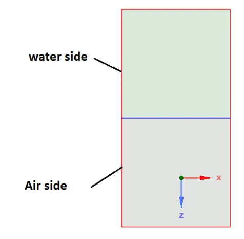
Draw 2 rectangle one above with dimension of 10mm X 20mm as shown below.

Make a surface using pull tool and enable share topology in work bench.

Mesh

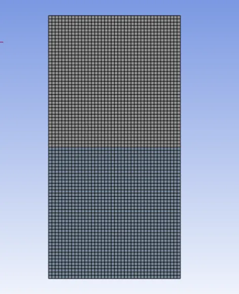
Element Size = 0.5mm

Setup

Solver

Pressure-based, Absolute, Transient

Gravity -9.81 m/s² acting in y direction.

Material

Fluid – Air & Water Liquid

Multiphase

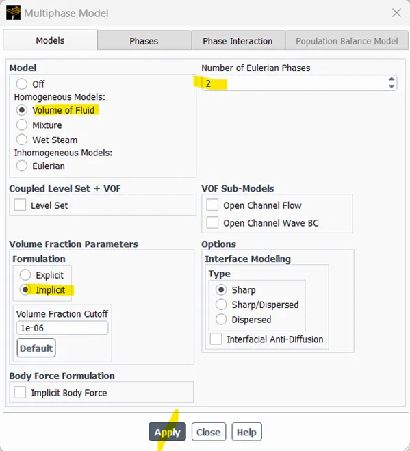
Phases

Air- Primary Phase

Water – Secondary Phase

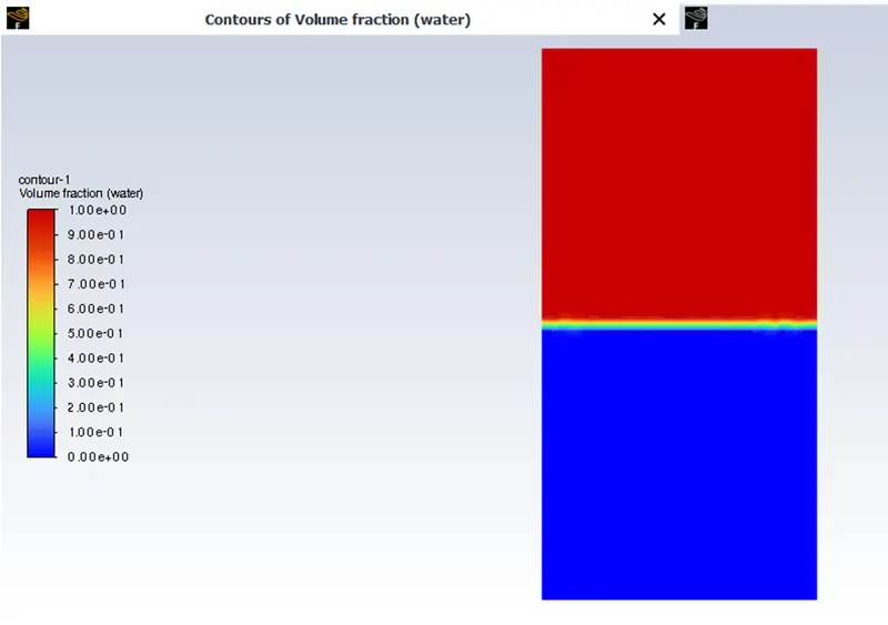
Run Standard initialization

Patch

Phase --> water

Variable --> Volume Fraction

Zones to Patch --> water_surface

Value --> 1

Hit Patch

Then select air surface in Zones to patch and give value 0 then hit Patch

Contour

Post Processing --> contours --> New --> contours of (Phases) --> Select all surfaces --> Volume Fraction --> water --> save and Display

Animation

Activities --> Create --> Solution Animation --> Animation Object --> Volume fraction --> ok

Run calculation

Time-step Method – Fixed

Time Step Size – 0.005

No.of time steps – 1500

Results

https://drive.google.com/file/d/1AoNnHxYB85w1EuU9LmZdx4SRja6115Ke/view?usp=sharing

Initial State of Volume Fraction

Final State of Volume Fraction

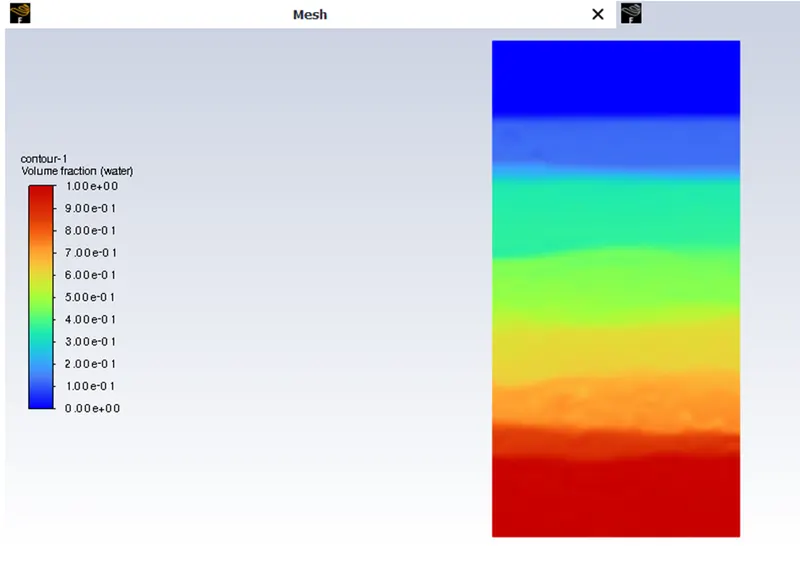
Results of Refined Mesh, with element size =0.3mm

Time Step Size = 0.003 s

https://drive.google.com/file/d/1cE7t81_D3kvle8HYNVYRI7d6ABIO_BhO/view?usp=share_link

Final State of Volume Fraction

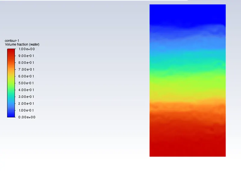
Results of Refined Mesh, with element size =0.3mm and User-defined Material

User-defined Material

Density = 400 kg/m³

Viscosity = 0.001 kg/m-s

Final State of Volume Fraction

https://drive.google.com/file/d/1SwdW1vYnM8lRwaavmvaPssSJqWSxt8sL/view?usp=sharing

Atwood number

The Atwood number, named after George Atwood, is a dimensionless parameter used in fluid dynamics to quantify the density difference between two fluids involved in a flow or wave phenomenon. It characterizes the buoyancy-driven flow and is often used in the context of studying instabilities such as Rayleigh-Taylor waves.

The Atwood number (A) is defined as the absolute value of the density difference between the two fluids divided by the sum of their densities. Mathematically, it can be expressed as:

A = |(ρ1 - ρ2)| / (ρ1 + ρ2)

where ρ1 and ρ2 are the densities of the two fluids.

The Atwood number ranges between 0 and 1, representing different density configurations:

• A = 0: Both fluids have the same density. There is no density difference, and the fluids are considered neutrally buoyant.
• A < 0: The lighter fluid is above the denser fluid, resulting in a stable configuration where buoyancy forces resist mixing.
• A > 0: The denser fluid is above the lighter fluid, leading to an unstable configuration that can result in mixing, wave formation, and instabilities such as Rayleigh-Taylor waves.

The Atwood number serves as a fundamental parameter in the analysis and modeling of buoyancy-driven flows and wave phenomena. It provides insights into the behavior of fluid instabilities, the growth rates of waves, and the overall dynamics of interfacial mixing. By varying the Atwood number, researchers can investigate different density configurations and understand the effects of density differences on flow behavior.

Material	Density for case 1	Density for case 2
Air	1.225	400
Water	998.2	998.2
Atwood Number	0.9975	0.4278

The variation in Atwood number has a significant influence on the behavior of instabilities, particularly in buoyancy-driven flows such as the Rayleigh-Taylor instability. Changes in the Atwood number can affect the growth rate, mixing dynamics, and overall behavior of the instability. Here's how the variation in Atwood number affects the behavior of the instability:

1. Growth Rate: The Atwood number directly affects the growth rate of the instability. In general, a higher Atwood number (larger density difference) leads to a faster growth rate of the instability. This is because a larger density difference creates a stronger buoyancy force, driving the fluids to mix more rapidly. Conversely, a lower Atwood number (smaller density difference) results in a slower growth rate as the buoyancy forces are relatively weaker.
2. Instability Structure: The Atwood number also influences the structure and characteristics of the instability. Higher Atwood numbers tend to produce more pronounced and larger-scale structures with significant mixing at the interface. The interfacial deformations, such as spikes and bubbles, become more prominent and can undergo complex interactions. In contrast, lower Atwood numbers may exhibit smaller-scale structures with reduced mixing effects.
3. Mixing Efficiency: The Atwood number affects the efficiency of mixing between the fluids. Higher Atwood numbers generally result in more efficient mixing due to the stronger buoyancy forces driving the interpenetration of the fluids. As a result, there is enhanced mass and momentum transfer across the interface, leading to faster and more thorough mixing. Lower Atwood numbers exhibit relatively slower and less efficient mixing.
4. Transition to Turbulence: At higher Atwood numbers, the Rayleigh-Taylor instability can transition to a turbulent flow regime more readily. The enhanced mixing and larger-scale deformations associated with higher Atwood numbers contribute to the development of turbulence. Turbulent flow introduces additional complexities, including enhanced energy dissipation, increased mixing rates, and altered flow dynamics.
5. Nonlinear Effects: Nonlinear effects become more pronounced with increasing Atwood numbers. As the instability grows, the interfacial dynamics and fluid motion become strongly nonlinear, leading to interactions between different modes and the development of secondary instabilities. These nonlinear effects can significantly influence the behavior of the instability and the subsequent flow evolution.

In summary, the variation in the Atwood number plays a crucial role in shaping the behavior of buoyancy-driven instabilities like the Rayleigh-Taylor instability. It affects the growth rate, instability structure, mixing efficiency, transition to turbulence, and nonlinear interactions. By manipulating the Atwood number, researchers can explore different regimes of instability behavior, enabling a better understanding of these phenomena and their implications in various applications.

Conclusion

Rayleigh Taylor instability simulation performed for 2 different mesh sizes with base mesh size 0.5 mm and refined mesh 0.3 mm. And another simulation done for refined mesh size with user defined material. Volume fraction animation file created for all 3 different simulation. Atwood number was calculated and the significant influence on the behavior of instabilities explained briefly.

In summary, the variation in the Atwood number plays a crucial role in shaping the behavior of buoyancy-driven instabilities like the Rayleigh-Taylor instability. It affects the growth rate, instability structure, mixing efficiency, transition to turbulence, and nonlinear interactions. By manipulating the Atwood number, researchers can explore different regimes of instability behavior, enabling a better understanding of these phenomena and their implications in various applications.