Week 12 - Validation studies of Symmetry BC vs Wedge BC in OpenFOAM vs Analytical H.P equation

Validation studies of Symmetry BC vs Wedge BC in OpenFOAM vs Analytical H.P Equation.

Aim:

Simulate an axi-symmetric flow by applying the wedge and Symmetry boundary condition in OpenFoam for different angles and write a code in Matlab to automate the generation of blockMeshDict file.

• Validate Hydro-dynamic length with numerical result.
• Validate the fully developed flow velocity profile with its analytical profile.
• Validate maximum velocity and pressured drop for fully developed flow.
• Highlight the difference in both boundary conditions in terms of their usage application.

Introduction:

OpenFOAM (Open Field Operation and Manipulation) is an open-source software for computational fluid dynamics (CFD) modeling. This report provides a detailed analysis of the simulation of flow through a pipe in OpenFOAM. The simulation will be performed to study the flow characteristics and its behavior in a pipe.

Problem Description:

The problem considered in this simulation is the flow of fluid through a pipe of length L and diameter D. Here we will simulate an axi-symmetric flow by applying the wedge and Symmetry boundary condition. The flow is laminar and flows through a constant cross-section pipe at an inlet Reynold’s number 2100.

The fluid is assumed to be incompressible and laminar with a constant viscosity. So we will perform steady state simulation and validate the results with Hagen-poiseuill’s equation.

The velocity profile at the inlet of the pipe is considered to be 0.01 m/s, and the pressure at the outlet is considered to be atmospheric. The simulation is performed to study the following result.

• Validating Hydro-dynamic length with the numerical result.
• Validating the fully developed flow velocity profile with its analytical profile.
• Validating maximum velocity and pressured drop for fully developed flow.
• Post-process Shear stress and validate wall shear stress for fully developed flow.

Hagen-Poiseuil’s equation:

Hagen-Poiseuille equation is a mathematical expression that describes the laminar flow of an incompressible fluid in a cylindrical pipe. The equation is derived from the Navier-Stokes equations, which describe the motion of fluid. The Hagen-Poiseuille equation predicts the pressure drop and flow rate through a pipe as a function of fluid viscosity, pipe diameter, length, and the pressure difference between the ends of the pipe.

It is only valid for laminar flow conditions, where the fluid moves in smooth and parallel layers, and not for turbulent flow conditions, where the fluid has chaotic and irregular movement.

The Hagen-Poiseuille equation is expressed as:

Q = (π * r^4 * ΔP) / (8 * μ * L)

where:

• Q is the flow rate through the pipe (m^3/s)
• r is the radius of the pipe (m)
• ΔP is the pressure drop across the pipe (Pa)
• μ is the dynamic viscosity of the fluid (Pa * s)
• L is the length of the pipe (m)

Note that this equation assumes that the fluid is incompressible, laminar, and Newtonian, and that the velocity of the fluid is uniform along the radial direction and is a maximum at the center of the pipe. It also assumes that the flow is fully developed, meaning that the velocity profile reaches a steady state before the fluid reaches the outlet of the pipe.

Hydrodynamic Length:

Hydrodynamic length, also known as the entrance length, is the length of the pipe required for the flow of fluid to reach a fully developed velocity profile. In other words, it is the distance required for the fluid to adjust to the pipe geometry and reach a steady state.

The hydrodynamic length can be calculated using the following equation:

Lh = 0.05 * Re * D

where:

• Lh is the hydrodynamic length (m)
• Re is the Reynolds number, a dimensionless number that describes the flow regime (laminar, transitional or turbulent)
• D is the diameter of the pipe (m)

Shear Stress:

The equation to calculate the shear stress at the wall of a pipe is:

τ = μ * dv/dy

where:

• τ is the shear stress at the wall (Pa or N/m^2)
• μ is the dynamic viscosity of the fluid (Pa * s)
• dv/dy is the velocity gradient perpendicular to the wall, which represents the rate of change of velocity in the direction perpendicular to the wall.

To validate the wall shear stress for fully developed flow, one can compare the calculated shear stress with the theoretical value for fully developed flow in a circular pipe.

Methodology:

1. Geometry and Mesh Generation: The pipe geometry is created using OpenFOAM's built-in CAD tools. The mesh file is generated using Matlab. The mesh quality is checked using checkMesh.
2. Case Setup: The simulation case is set up in OpenFOAM by defining the governing equations, boundary conditions, and initial conditions. The flow is modeled using the Navier-Stokes equations.
3. Solver Selection: A suitable solver is selected from OpenFOAM's library of solvers to solve the governing equations. The icoFoam solver is used in this simulation.
4. Running the Simulation: The simulation is run using the OpenFOAM run script. The solution is monitored and checked for convergence.
5. Post-Processing: The results of the simulation are post-processed using ParaView, an open-source visualization tool. The velocity and pressure distribution along the pipe length are analyzed.

Input Values:

Diameter of the Pipe (d)= 0.04

Wedge angle (theta) = 10, 25, 45 (in degree)

Renold’s number(Re) = 2100

Density of the fluid(rho) = 997 kg/m^3

Dynamic Viscosity of water (mu) = 0.00089 Ns/m^2 or (Pa.s)

Kinematic Viscosity (nu) =(mu)/rho

Formulas:

Hydrodynamic Length(Lh) = 0.05 * Re *d = 4.2 m

Total Length of the pipe (L) = Lh + 1.54 = 5.74 m

%creating blockMeshDict file for OpenFoam

d=0.04 %in meters, assumed

r=d/2;

theta=4

Re=2100

rho=997; % in kg/m^3

L_etr=0.06*Re*d;

L=L_etr+0.7;

mu=0.00089; % viscosity of water

nu=mu/rho; % kinetic viscosity

% boundary conditions

v_avg= Re*nu/d

v_max=2*v_avg;

deltap= (8*v_avg*mu*L)/r^2;

% calculating shear stress

R = linspace(0,(d/2),1000);

for i = 1:length(R)

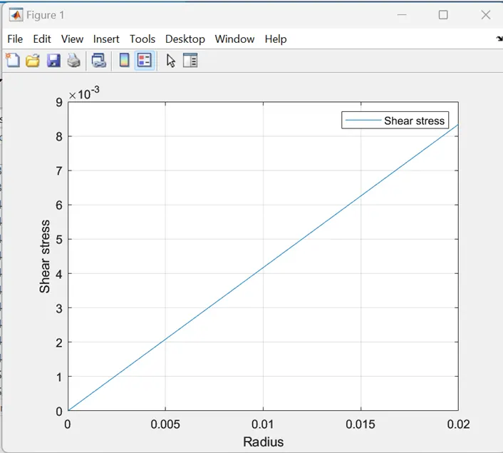
tau(i) = 2*mu*v_max*(abs(R(i)))/r^2

end

plot(R,tau)

xlabel('Radius')

ylabel('Shear stress')

grid on

legend ('Shear stress');

h1='/*----------------------------------*- C++ -*------------------------------------*\\';

h2=' ========= | ';

h3=' \\\\ / F ield | OpenFOAM: The Open Source CFD Toolbox ';

h4=' \\\\ / O peration | Website: https://openfoam.org ';

h5=' \\\\ / A nd | Version: 7 ';

h6=' \\\\/ M anipulation | ';

h7='\\*----------------------------------------------------------------------------------*/';

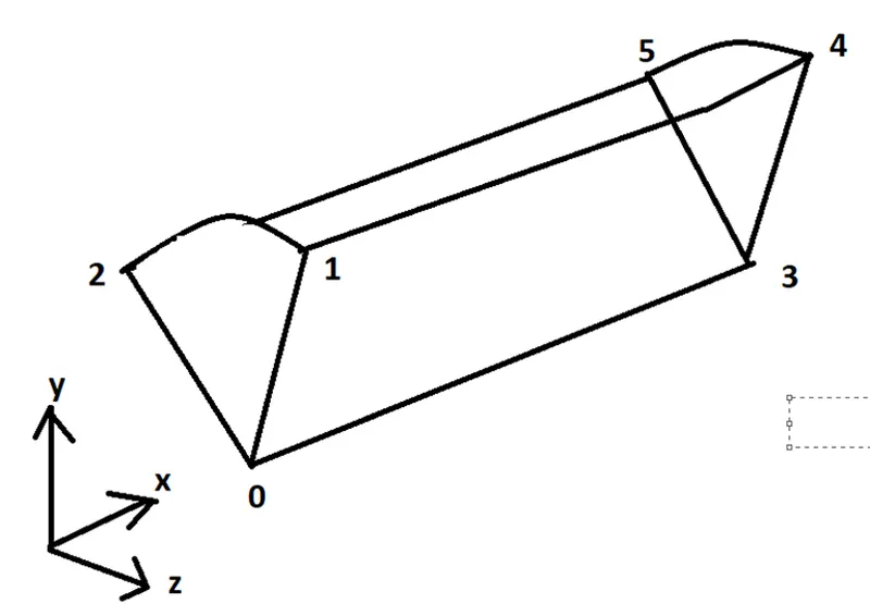
v0=[0 0 0]

v1=[0 r*cosd(theta/2) r*sind(theta/2)]

v2=[0 r*cosd(theta/2) -r*sind(theta/2)]

v3=[L 0 0]

v4=[L r*cosd(theta/2) -r*sind(theta/2)]

v5=[L r*cosd(theta/2) r*sind(theta/2)]

f1=fopen('blockMeshDict.txt','w')

fprintf(f1,'%s\n',h1);

fprintf(f1,'%s\n',h2);

fprintf(f1,'%s\n',h3);

fprintf(f1,'%s\n',h4);

fprintf(f1,'%s\n',h5);

fprintf(f1,'%s\n',h6);

fprintf(f1,'%s\n',h7);

fprintf(f1, 'FoamFile\n');

fprintf(f1, '{\n');

fprintf(f1, ' format ascii;\n');

fprintf(f1, ' class dictionary;\n');

fprintf(f1, ' object blockMeshDict;\n');

fprintf(f1, '}\n');

fprintf(f1, '// * * * * * * * * * * * * * * * * * * * * * * * * * * * * * * * * * * * * * //\n');

fprintf(f1, 'convertToMeters 1;\n\n')

fprintf(f1, 'vertices\n(\n');

fprintf(f1, '\t (%d %d %d)\n', v0);

fprintf(f1, '\t (%d %d %d)\n', v1);

fprintf(f1, '\t (%d %d %d)\n', v2);

fprintf(f1, '\t (%d %d %d)\n', v3);

fprintf(f1, '\t (%d %d %d)\n', v4);

fprintf(f1, '\t (%d %d %d)\n', v5);

fprintf(f1,');\n\n');

fprintf(f1,'blocks\n(\n');

fprintf(f1,'\t hex(0 1 2 0 3 4 5 3) (300 300 1) simpleGrading (1 0.1 0)\n);\n\n');

fprintf(f1,'edges\n(\n');

fprintf(f1,'\t arc 1 2 (0 %.6e 0)\n', r);

fprintf(f1,'\t arc 4 5 (%d %.6e 0)\n', L, r);

fprintf(f1,');\n\n');

fprintf(f1,['boundary\n(\n\t axis\n\t\t{\n\t\t type empty;\n\t\t faces\n\t\t (\n']);

fprintf(f1,'\t\t\t (0 3 3 0)\n\t\t );\n\t\t}\n');

fprintf(f1,['\t wall\n\t\t{\n\t\t type wall;\n\t\t faces\n\t\t (\n']);

fprintf(f1,'\t\t\t (2 5 4 1)\n\t\t );\n\t\t}\n');

fprintf(f1,['\t inlet\n\t\t{\n\t\t type patch;\n\t\t faces\n\t\t (\n']);

fprintf(f1,'\t\t\t (0 0 2 1)\n\t\t );\n\t\t}\n');

fprintf(f1,['\t outlet\n\t\t{\n\t\t type patch;\n\t\t faces\n\t\t (\n']);

fprintf(f1,'\t\t\t (3 4 5 3)\n\t\t );\n\t\t}\n');

fprintf(f1,['\t wedgeFront\n\t\t{\n\t\t type wedge;\n\t\t faces\n\t\t (\n']);

fprintf(f1,'\t\t\t (0 3 5 2)\n\t\t );\n\t\t}\n');

fprintf(f1,['\t wedgeBack\n\t\t{\n\t\t type wedge;\n\t\t faces\n\t\t (\n']);

fprintf(f1,'\t\t\t (0 1 4 3)\n\t\t );\n\t\t}\n);\n');

fprintf(f1, 'mergePatchPairs')

fprintf(f1,'\n(\n);\n')

fprintf(f1,'// ************************************************************************* //')

% % fprintf(fileID, '\t arc 1 2 (0 2.000000e-03 0)\n');

% fprintf(fileID, '\t arc 1 2 (0 %.6e 0)\n', r);

fclose(f1);

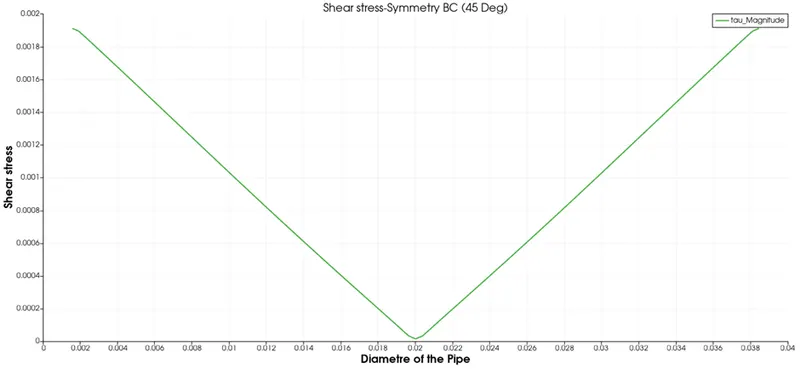
Shear Stress Plot along the Radius of the Pipe

blockMeshDict file for wedge angle 10 degree

/*--------------------------------*- C++ -*----------------------------------*\

========= |

\\ / F ield | OpenFOAM: The Open Source CFD Toolbox

\\ / O peration | Website: https://openfoam.org

\\ / A nd | Version: 9

\\/ M anipulation |

\*---------------------------------------------------------------------------*/

FoamFile

{

format ascii;

class dictionary;

object blockMeshDict;

}

// * * * * * * * * * * * * * * * * * * * * * * * * * * * * * * * * * * * * * //

convertToMeters 1;

vertices

(

(0 0 0)

(0 -1.743115e-03 1.992389e-02)

(0 1.743115e-03 1.992389e-02)

(5.740000e+00 0 0)

(5.740000e+00 -1.743115e-03 1.992389e-02)

(5.740000e+00 1.743115e-03 1.992389e-02)

);

blocks

(

hex (0 3 3 0 1 4 5 2) (100 1 50) simpleGrading (1 1 1)

);

edges

(

arc 1 2 (0 0 0.02)

arc 4 5 (5.74 0 0.02)

);

boundary

(

axis

{

type empty;

faces

(

(0 3 3 0)

);

}

fixedWalls

{

type wall;

faces

(

(1 4 5 2)

);

}

front

{

type wedge;

faces

(

(0 2 5 3)

);

}

back

{

type wedge;

faces

(

(0 3 4 1)

);

}

inlet

{

type patch;

faces

(

(0 1 2 0)

);

}

outlet

{

type patch;

faces

(

(3 5 4 3)

);

}

);

mergePatchPairs

(

);

// ************************************************************************* //

Replace the vertices with the following data for angles 25 and 45.

Vertices for wedge angle 25 degree

(0 0 0)

(0 1.952592e-02 4.328792e-03)

(0 1.952592e-02 -4.328792e-03)

(5.740000e+00 0 0)

(5.740000e+00 1.952592e-02 4.328792e-03)

(5.740000e+00 1.952592e-02 -4.328792e-03)

Vertices for Wedge angle 45 degree

(0 0 0)

(0 1.847759e-02 7.653669e-03)

(0 1.847759e-02 -7.653669e-03)

(5.740000e+00 0 0)

(5.740000e+00 1.847759e-02 7.653669e-03)

(5.740000e+00 1.847759e-02 -7.653669e-03)

And for Symmetry boundary condition we need to replace Symmetry in the place of wedge in the blockMesh Dict, Velocity and Pressure files.

Pressure File

/*--------------------------------*- C++ -*----------------------------------*\

========= |

\\ / F ield | OpenFOAM: The Open Source CFD Toolbox

\\ / O peration | Website: https://openfoam.org

\\ / A nd | Version: 10

\\/ M anipulation |

\*---------------------------------------------------------------------------*/

FoamFile

{

format ascii;

class volScalarField;

object p;

}

// * * * * * * * * * * * * * * * * * * * * * * * * * * * * * * * * * * * * * //

dimensions [0 2 -2 0 0 0 0];

internalField uniform 0;

boundaryField

{

inlet

{

type zeroGradient;

}

outlet

{

type fixedValue;

value uniform 1;

}

fixedWalls

{

type zeroGradient;

}

front

{

type wedge;

}

back

{

type wedge;

}

axis

{

type empty;

}

}

// ************************************************************************* //

Velocity File

/*--------------------------------*- C++ -*----------------------------------*\

========= |

\\ / F ield | OpenFOAM: The Open Source CFD Toolbox

\\ / O peration | Website: https://openfoam.org

\\ / A nd | Version: 10

\\/ M anipulation |

\*---------------------------------------------------------------------------*/

FoamFile

{

format ascii;

class volVectorField;

object U;

}

// * * * * * * * * * * * * * * * * * * * * * * * * * * * * * * * * * * * * * //

dimensions [0 1 -1 0 0 0 0];

internalField uniform (0 0 0);

boundaryField

{

inlet

{

type fixedValue;

value uniform (0.01 0 0);

}

outlet

{

type zeroGradient;

}

fixedWalls

{

type noSlip;

}

front

{

type wedge;

}

back

{

type wedge;

}

axis

{

type empty;

}

}

// ************************************************************************* //

ControlDict file

/*--------------------------------*- C++ -*----------------------------------*\

========= |

\\ / F ield | OpenFOAM: The Open Source CFD Toolbox

\\ / O peration | Website: https://openfoam.org

\\ / A nd | Version: 10

\\/ M anipulation |

\*---------------------------------------------------------------------------*/

FoamFile

{

format ascii;

class dictionary;

location "system";

object controlDict;

}

// * * * * * * * * * * * * * * * * * * * * * * * * * * * * * * * * * * * * * //

application icoFoam;

startFrom startTime;

startTime 0;

stopAt endTime;

endTime 60;

deltaT 0.01;

writeControl timeStep;

writeInterval 20;

purgeWrite 0;

writeFormat ascii;

writePrecision 6;

writeCompression off;

timeFormat general;

timePrecision 6;

runTimeModifiable true;

// ************************************************************************* //

Physical Properties File

/*--------------------------------*- C++ -*----------------------------------*\

========= |

\\ / F ield | OpenFOAM: The Open Source CFD Toolbox

\\ / O peration | Website: https://openfoam.org

\\ / A nd | Version: 10

\\/ M anipulation |

\*---------------------------------------------------------------------------*/

FoamFile

{

format ascii;

class dictionary;

location "constant";

object physicalProperties;

}

// * * * * * * * * * * * * * * * * * * * * * * * * * * * * * * * * * * * * * //

nu [0 2 -1 0 0 0 0] 1e-06;

// ************************************************************************* //

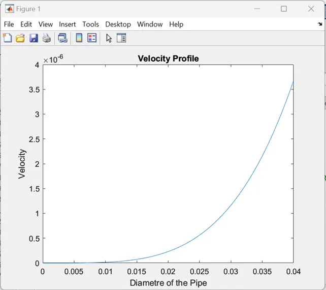
Matlb Code to find the Velocity Profile

clear all

close all

clc

D = 0.04; % pipe diameter [m]

U = 0.0937312; % fluid velocity [m/s]

mu = 0.00089; % fluid dynamic viscosity

R = D/2; % pipe radius [m]

rho = 997 % Density of water

nu =mu/rho % Kinematic Viscosity

Re = 2100; % Reynolds number

d = linspace(0,D,50); % radial coordinate

%

% % % calculate velocity

u = zeros(size(d));

for i = 1:length(d)

u(i) = 4.081896*(22/7)*(1/16)*d(i)^4/(128*mu*4.9)

end

plot(u, d)

title('Velocity Profile')

xlabel('Velocity')

ylabel('Diametre of the Pipe')

To calculate the velocity Profile along the diameter of the Pipe we need to mirror the geometry with respect to axis of symmetry that is the axis passes along the centre of the pipe throughout the length.

Mirror Results in ParaView:

Step 1: Choose the Filter

Go to Filters, Alphabetical and Search. If the filter is disabled/not visible it can be accessed using Filters and search and then typing name Reflect in the search window.

Step 2: Select the Symmetry of the Plane

We want to reflect about the central axis which is the bottom edge of the wedge. It is important to make note of the coordinate axes before selecting the symmetry plane. In this case, the bottom edge of the wedge is aligned to the central axis of the flow and since that is axis of symmetry, we want to choose the Y-plane that passes through the symmetry axis.

And as the Y- coordinate is minimum for the bottom edge of the wedge, we choose the symmetry plane as Y Min.

Step 3: Click on the Apply button

By clicking on the apply button, we can see the complete 2D solution for our problem. The solution has been mirrored about the central axis. Now, we can use the plot over line tool to visualize the velocity profile across the complete diameter. The velocity profile appears as shown below.

Calculating the Shear stress Value in ParaView

Step 1 : Computing the Magnitude of vector field U using Calculator Tool

1. Make sure that the common toolbar under view tab is enabled.

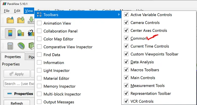
2.Click on the Calculator tool that can be found in the extreme left of the commom toolbar.

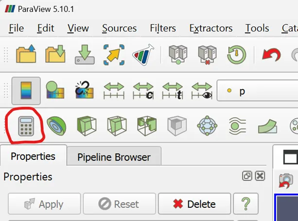
3. A calculator will appear in the properties box on the left pane of the Paraview window.
4. In the calculator, we want to compute the magnitude of the U vector, so type mag(U) inside the calculation box . Vectors button can also be used to select U. The result of the computation is stored inside that name so that it can be accessed later. In the above picture, mag_ U is the result array name.

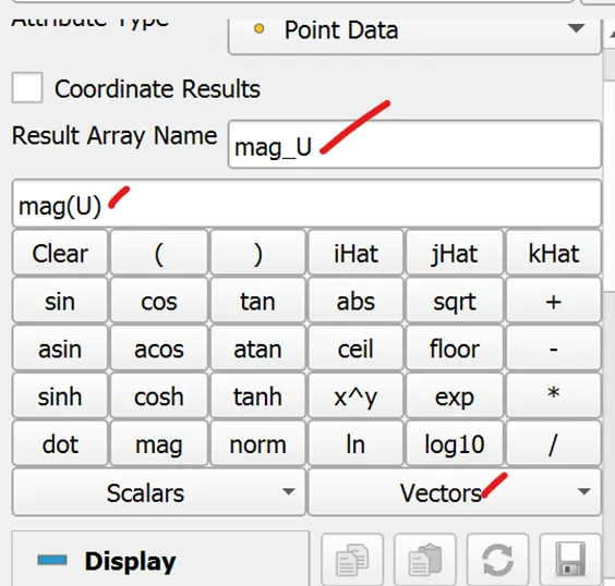
5. On clicking on the apply button, the magnitude of the velocity vector U is computed and applied in the Field Variable selection box.

Step 2: Computing the Gradients for U_magnitude using the ‘Gradients ‘ tool.

1. Now we need to compute the gradients of U_magnitude inside the entire domain, since velocity gradient is what determines the shear stress developed inside the fluid.
2. This can be done using the “ Gradients “ tool inside Filter.

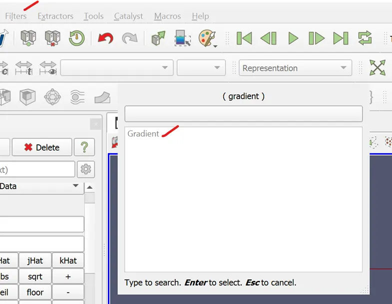
3. The properties windows shows as follows.

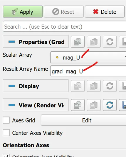
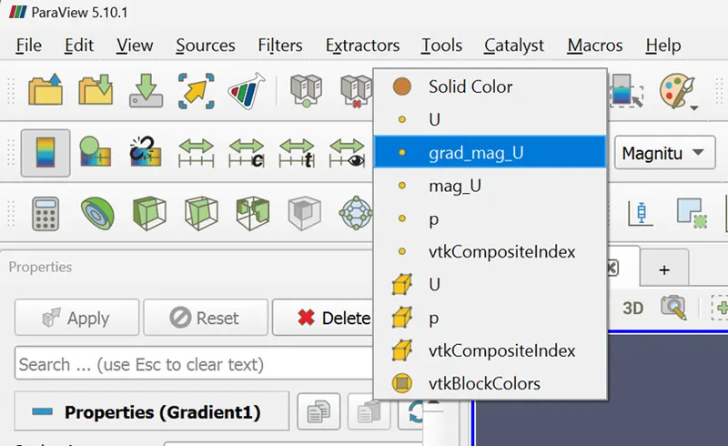
4. In the Scalar Array box, select the array name where the U_magnitude values were previously stored. Since, we stored the results inside mag_U, that quantity is selected as the Scalar Array in the above picture.
5. Type the result array name as desired. That is where the gradients of U_magnitude values will be stored, so that we can access them in the future. In the above picture grad_mag_U is the array name chosen for that purpose.
6. Clicking on the Apply button will create a new quantity of the specified name inside the Field Variable Selection box.

Step 3: Computing the Shear-stress quantity

1. In the previous step, we computed the velocity gradients data. Now we need to use the formula for shear stress to calculate it.

The equation to calculate the shear stress at the wall of a pipe is:

τ = μ * dv/dy

where:

• τ is the shear stress at the wall (Pa or N/m^2)
• μ is the dynamic viscosity of the fluid (Pa * s)
• dv/dy is the velocity gradient perpendicular to the wall, which represents the rate of change of velocity in the direction perpendicular to the wall.

2. Therefore, we can obtain shear stress by multiplying the velocity gradient with the dynamic viscosity of the fluid under study.
3. Assuming water is our working fluid, and that is at the room temperature 25 C, the dynamic viscosity is 0.00089 Ns/m^2.
4. Now click on the calculator, and select our velocity gradient vector array by clicking on the vectors button on the bottom-right and then multiply that by dynamic viscosity as shown in the picture below.

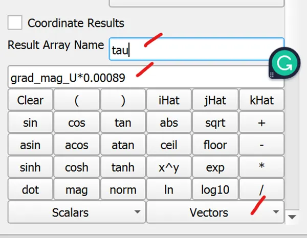
5. We have used the variable tau to store shear stress date.

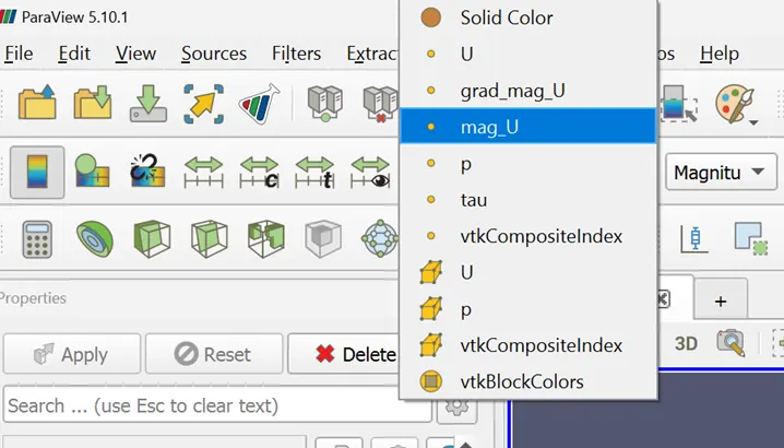
6.Clicking on the apply button will create a new quantity inside the Field Variable selection box as shown below.

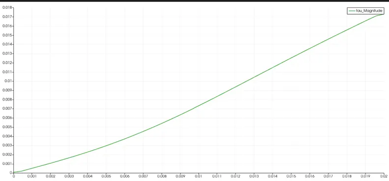
Step-4: Plotting Shear-stress

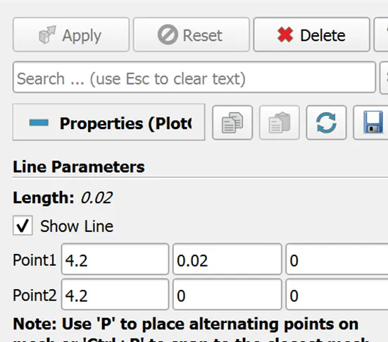
We can create the Plot Over Line tool located in the common toolbar.

Results

1. Validating Hydrodynamic Length with the numerical result.

Hydrodynamic length = 0.05 * Re * d = 0.05 *2100 * 0.04 => 4.2 m

2. Velocity and Shear stress Plot for Wedge Boundary condition with the angle of 10 degree.

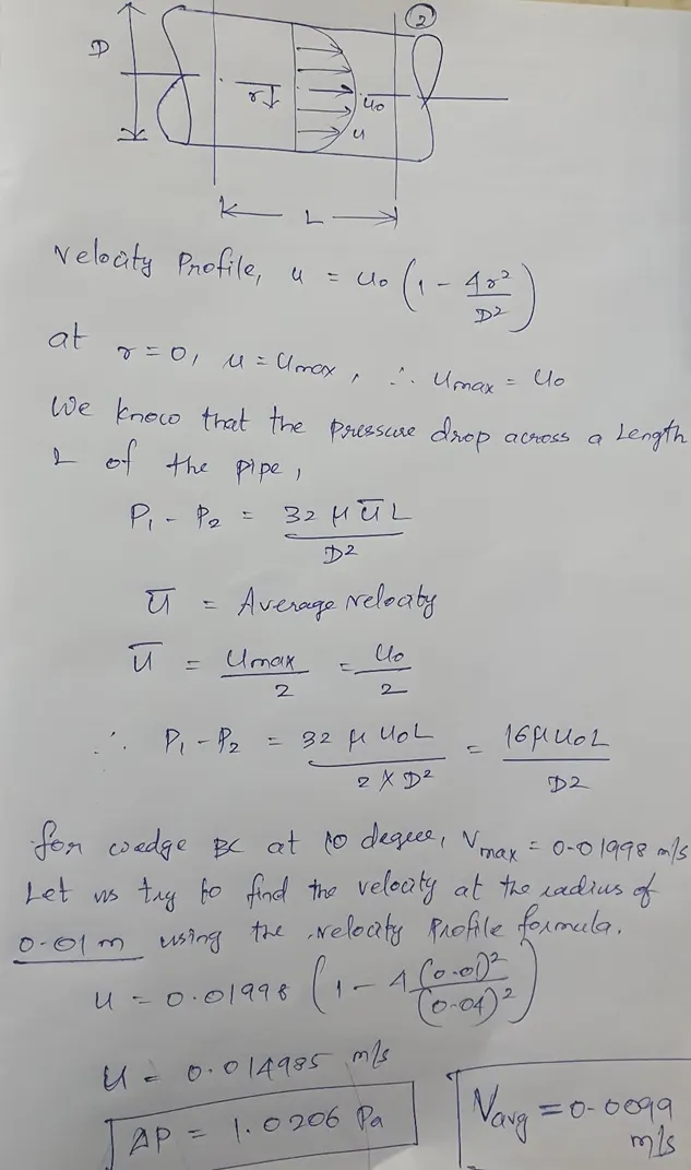
V_max = 0.01998

Courant Number = Velocity x dt/dx => 0.01 X 0.1/(5.74/100)

C = 0.0174

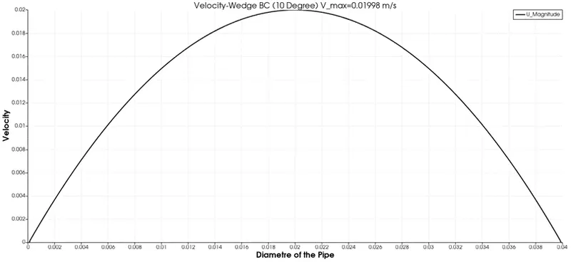
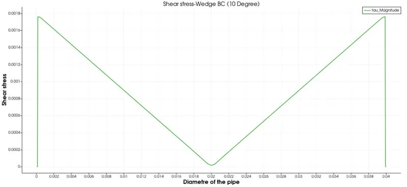
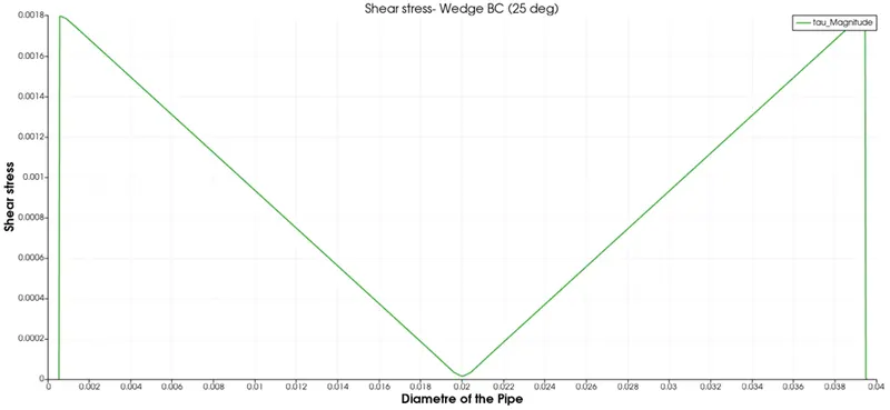
Velocity and Shear stress Plot for Wedge Boundary condition with the angle of 25 degree.

V_max = 0.019984 m/s

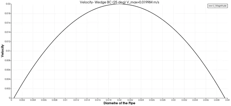
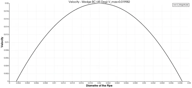
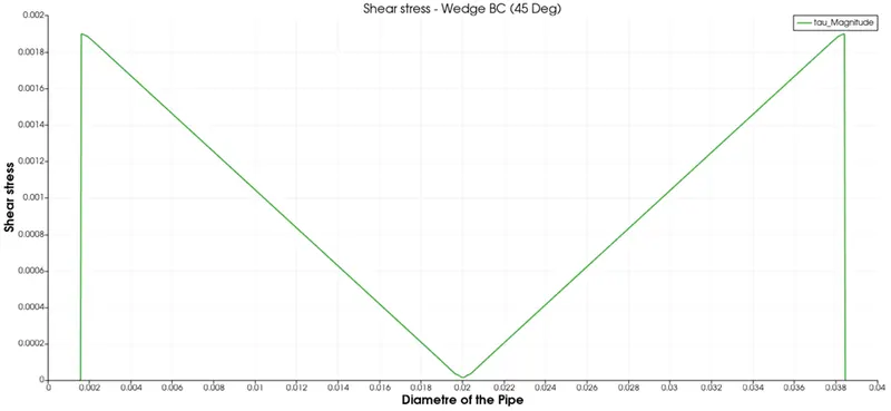
Velocity and Shear stress Plot for Wedge Boundary condition with the angle of 45 degree.

V_max = 0.019982 m/s

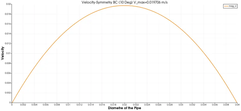
3. Velocity and Shear stress Plot for Symmetry Boundary condition with the angle of 10 degree.

V_max = 0.019706 m/s

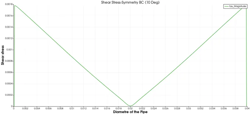
Velocity and Shear stress Plot for Symmetry Boundary condition with the angle of 25 degree.

V_max = 0.01976 m/s

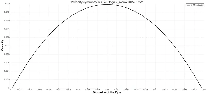
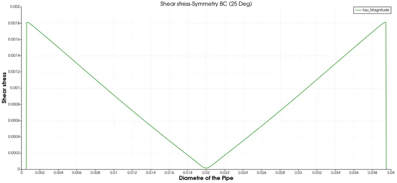
Velocity and Shear stress Plot for Symmetry Boundary condition with the angle of 45 degree.

V_max = 0.0198514 m/s

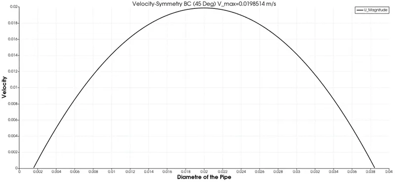
V_max

BC	Angle
	10	25	45
Wedge	0.01998 m/s	0.019984 m/s	0.019982 m/s
Symmetry	0.019706 m/s	0.01976 m/s	0.0198514 m/s

Velocity Profile- Matlab

4. Pressure Drop = P1- P2 = 16*mu*v_max*L/D^2

= 16* 0.00089*0.01998*5.74/(0.04)^2

= 1.0206 Pa

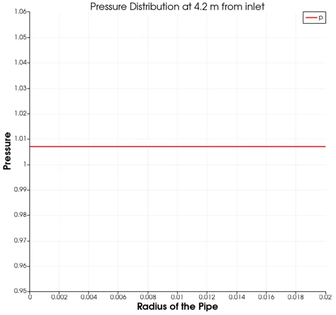
Pressure is constant along the cross section for a flow through a circular pipe due to the symmetry of the pipe. The pressure exerted by the fluid on the walls of the pipe is normal to the wall at every point, which implies that there is no variation in the pressure in the radial direction of the pipe. Therefore, the pressure remains constant along any cross section of the pipe.

This result is a consequence of the continuity equation, which states that the mass flow rate of a fluid through a pipe is conserved. In order for the mass flow rate to be conserved, the velocity of the fluid must vary inversely with the cross-sectional area of the pipe. This inverse variation of velocity and area is what leads to the constancy of pressure along the cross section of the pipe.

This phenomenon is known as Poiseuille's law, and it is widely used to model fluid flow through circular pipes.

Difference Between Wedge and Symmetry Boundary Condition

1. Wedge boundary condition:

A wedge boundary condition is typically used to simulate a flow around a body with a sharp edge or corner. This type of boundary condition is often applied to the edges of a computational domain where a solid object is present, such as an aircraft wing or a submarine hull. A wedge boundary condition is often used to simulate a no-slip condition, meaning that the velocity of the fluid is zero at the surface of the solid object. This type of boundary condition is important for accurately predicting the behavior of the fluid around the solid object, such as the drag force and the lift force.

2. Symmetry boundary condition:

A symmetry boundary condition is typically used to model a situation where the flow is symmetric with respect to a plane or an axis of symmetry. This type of boundary condition is often applied to a plane that divides the computational domain into two halves that are mirror images of each other. By imposing a symmetry boundary condition, only one-half of the domain needs to be simulated, which reduces the computational cost of the simulation. A symmetry boundary condition is often used to model situations where the flow is symmetric, such as in a wind tunnel where the flow is expected to be symmetric with respect to the centerline of the tunnel.

In summary, a wedge boundary condition is used to simulate a no-slip condition around a solid object with a sharp edge or corner, while a symmetry boundary condition is used to reduce the computational cost of a simulation by modeling a situation where the flow is symmetric with respect to a plane or an axis of symmetry.