Week 7 - Simulation of a 1D Supersonic nozzle flow simulation using Macormack Method

Simulation of a 1D Supersonic nozzle flow simulation using Maccormack Method

Aim

Simulate the isentropic flow through a quasi 1D subsonic-supersonic nozzle using MacCormak’s technique and get the following plots.

• Steady-state distribution of primitive variables inside the nozzle.
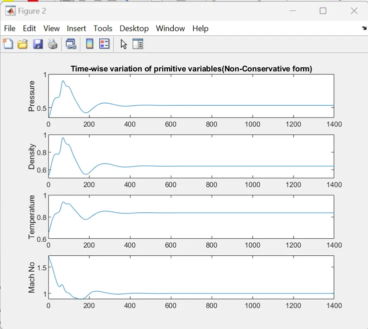
• Time-wise variation of primitive variables.
• Variation of Mass flow rate distribution inside the nozzle at different time steps during the time-marching process.
• Comparison of normalized mass flow rate distributions of both forms.

Quasi 1D Subsonic-Supersonic isentropic Nozzle Flow

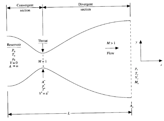
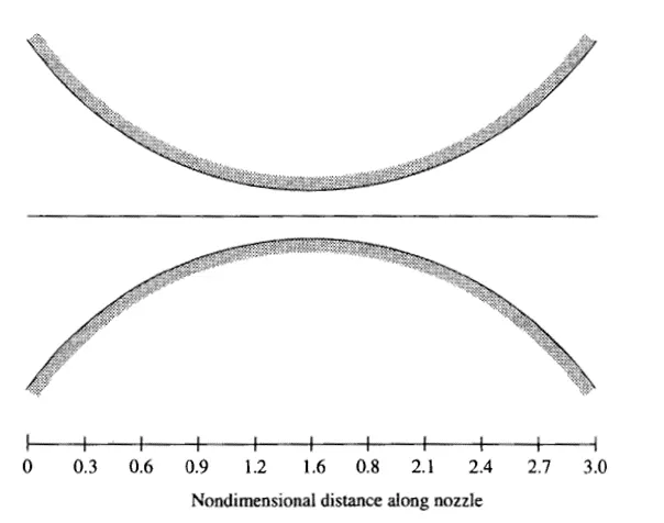
Consider a steady, isentropic flow through a CD nozzle as given in the figure.

The Pressure and temperature at the inlet is denoted by P₀ and T₀. The flow at the inlet to the nozzle comes from the reservoir, the cross-sectional area of the reservoir is large, and hence the velocity is small. The flow expands isentropically to supersonic speeds at the nozzle exit, where the exit pressure, temperature, velocity and Mach number are denoted by P_e, T_e, V_e, M_e respectively. The flow is locally subsonic in the convergent section of the nozzle, sonic at the throat and supersonic at the divergent section. The sonic flow values of pressure and temperature are denoted by P*, T* . The area of the sonic throat is denoted by A*.

The term "quasi 1D" refers to the assumption that the flow through the nozzle is one-dimensional, which is a simplification used to make the analysis and design of the nozzle easier. We make the assumption that the flow properties vary only with x-axis; this is tantamount to assuming uniform flow properties across any given cross section. Such flow is defined as quasi-one-dimensional flow.

The Governing Equations

Continuity: `rho<sub>1</sub> *A<sub>1</sub>*V<sub>1</sub> = rho<sub>2</sub>. A<sub>2</sub>. V<sub>2</sub>`

Momentum: `P<sub>1</sub>*A<sub>1</sub>+rho<sub>1</sub>*V<sub>1</sub>^2*A<sub>1</sub>+int P *dA = P<sub>2</sub>*A<sub>2</sub> + rho<sub>2</sub> * V<sub>2</sub>^2*A<sub>2</sub>`

Energy: `h<sub>1</sub>+(V<sub>1</sub>^2)/2 = h<sub>2</sub>+(V<sub>2</sub>^2)/2`

MacCormack method

The MacCormack method is a finite-difference method used to solve hyperbolic partial differential equations. It is an efficient and accurate method that is commonly used to simulate supersonic flow.

The simulation was carried out using the MacCormack method, which is a two-step algorithm. The first step is called the predictor step, where the solution is advanced in time using a forward difference scheme. The second step is called the corrector step, where the solution is corrected using a backward difference scheme. This two-step process ensures the stability of the simulation.

Steps:

Predictor step: ꝺf / ꝺt_p - Use forward difference for space terms

Solution update: f* = f_initial + ꝺf/ꝺt_p (∆t)

Corrector step: ꝺf*/ ꝺt_c – Use Backward difference for Space terms

Average Value : ꝺf / ꝺt_avg = 0.5 ( ꝺf/ꝺt_{p +} ꝺf/ꝺt_c )

Governing Equation- Non-conservative form

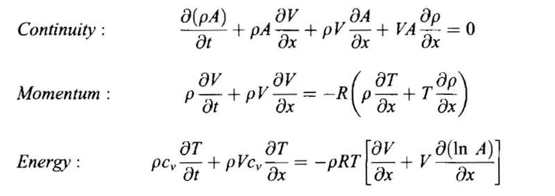
For nozzle flows, the flow-field variables are frequently expressed in terms of nondimensional variables, where the flow variables are referenced to their reservoir values. The non-dimensional variables ρ/ρ₀ , P/P₀ , and T/T₀ vary between 0 and 1, which is an "aesthetic" advantage when presenting the results.

Reservoir temperature and density are denoted by T₀ and ρ₀ , respectively, we define the non-dimensional temperature and density, respectively, as

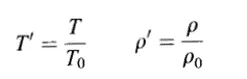
Here the prime denotes a dimensionless variable. Moreover, letting L denote the length of the nozzle, we define a dimensionless length as

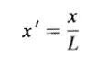
Denoting the speed of sound in the reservoir as a₀, where

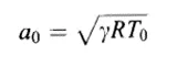
we define a dimensionless velocity as

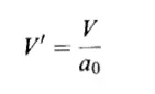
Also, the quantity L/a₀ has the dimension of time, and we define a dimensionless time as

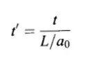
Finally, we ratio the local area A to the sonic throat area A* and define a dimensionless area as

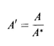
After applying non-dimensional variables governing equations become

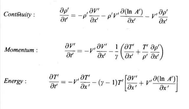
Applying the forward differencing in the above equations, we do the predictor step of the Maccormack method.

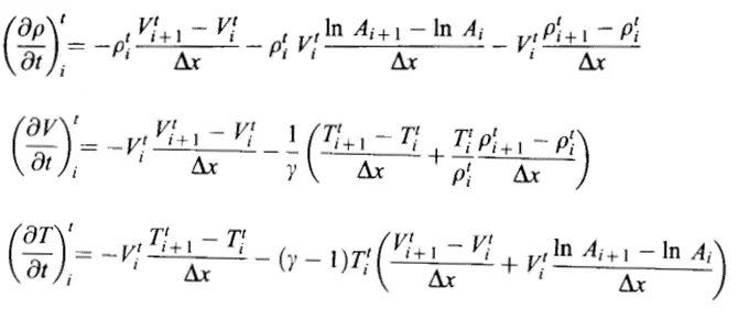
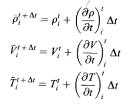
Predicted Values of flow field Variables

Corrector Step

Use Backward Differencing in the governing equations,

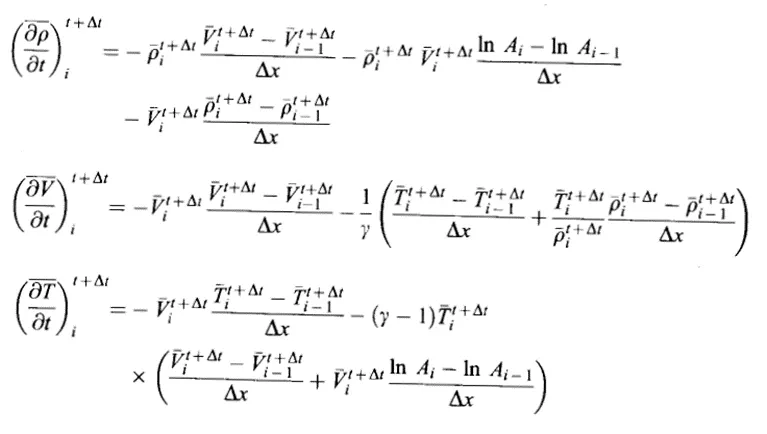
Finding Average Value

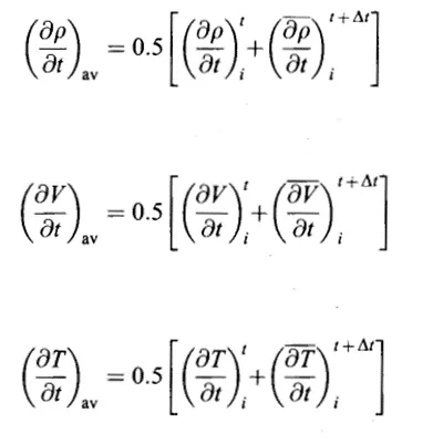
Corrector Values of Flow field Variables

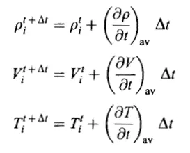
Calculation of Time step

The subsonic-supersonic isentropic nozzle flow is governed by nonlinear partial differential Equations. In this case, the exact stability criteria for a linear equation is that courant number less than 1.

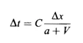
The above equation is the Courant Friedrichs-Lowry ( CFL) criterion for a one-dimensional flow, where V is the local flow velocity at a point in the flow and a is the local speed of sound, along with C< 1, simply states that ∆t must be less than, or at best equal to, the time it takes a sound wave to move from one grid point to the next.

At each grid point ∆t value will be different, so we use the following formula to calculate ∆t and use this value at all grid points.

Boundary Condition

We use method of characteristic to decide the number of variables to be fixed/ float at the inlet and outlet.

The method of characteristics tells us that at a boundary where one characteristic propagates into the domain, then the value of one dependent flow-field variable must be specified at that boundary, and if one characteristic line propagates out of the domain, then the value of another dependent flow-field variable must be allowed to float at the boundary; i.e., it must be calculated in steps of time as a function of the timewise solution of the flow field.

In conclusion at the subsonic inflow boundary, we must stipulate the values of two dependent flow-field variables, whereas the value of one other variable must be allowed to float. At the outlet, all flow field variables are allowed to float, as both characteristic lines move out of the boundary.

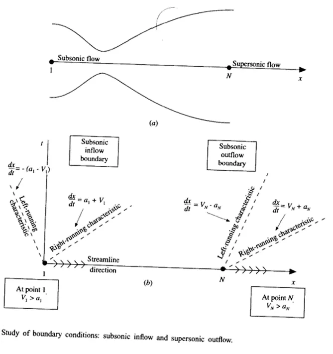
Inlet Boundary condition

We choose the velocity V₁, because on a physical basis we know the mass flow through the nozzle must be allowed to adjust to the proper steady state, and allowing V₁ to float makes the most sense as part of this adjustment. The value of V₁ changes with time and is calculated from information provided by the flow-field solution over the internal points, ( The internal points are those not on a boundary, i.e,, points 2 through N – 1 ), We use linear extrapolation from points 2 and 3 to calculate V₁. Here, the slope of the linear extrapolation line is determined from points 2 and 3 as

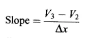
Using this slope to find V1 by linear extrapolation, we have

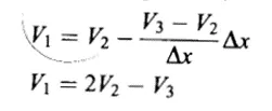
All other flow field variables are specified.

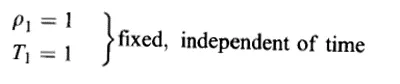
Outlet Boundary Condition

We allow all flow field variables to float.

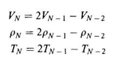
Nozzle Shape

The nozzle shape, A = A(x), is specified and held fixed, independent of time, section. We choose a parabolic area distribution given by,

Note that x = 1.5 is the throat of the nozzle, that the convergent section occurs for x < 1.5, and that the divergent section occurs for x > 1.5.

Initial Condition

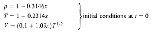
As density and Temperature decreases and V increases as the flow expands through the nozzle, we choose initial conditions that qualitatively behave in the same fashion. Let us assume linear variations of the flow-field variables, as a function of x.

Matlab code for Non-conservative form

clear

close all

clc

% non-conservative form

% inputs

n=31;

x=linspace(0, 3, n);

dx=x(2)-x(1);

gamma=1.4;

% calculate initial profiles

rho = 1-0.3146*x; % density

t=1-0.2314*x; % t= temperature

v=(0.1+1.09*x).*t.^0.5; % velocity

% area

a=1+2.2*(x-1.5).^2;

throat =find(a == 1);

% Time steps

nt=1400;

CFL=0.5;

dt=min((CFL.*dx)./(v+sqrt(t)));

% Outer time loop

for k=1:nt

rho_old=rho;

v_old= v;

t_old=t;

% Predictor method

for j=2:n-1

dvdx=(v(j+1)-v(j))/dx;

drhodx=(rho(j+1)-rho(j))/dx;

dtdx=(t(j+1)-t(j))/dx;

dlogadx=(log(a(j+1))-log(a(j)))/dx;

% Continuity equation

drhodt_p(j)=-rho(j)*dvdx-rho(j)*v(j)*dlogadx-v(j)*drhodx;

% Momentum equation

dvdt_p(j)=-v(j)*dvdx-(1/gamma)*(dtdx+(t(j)/rho(j))*drhodx);

% Energy equation

dtdt_p(j)=-v(j)*dtdx-(gamma-1)*t(j)*(dvdx+v(j)*dlogadx);

% solution update

rho(j)=rho(j)+drhodt_p(j)*dt;

v(j)=v(j)+dvdt_p(j)*dt;

t(j)=t(j)+dtdt_p(j)*dt;

end

% corrector method

for j=2:n-1

dvdx=(v(j)-v(j-1))/dx;

drhodx=(rho(j)-rho(j-1))/dx;

dtdx=(t(j)-t(j-1))/dx;

dlogadx=(log(a(j))-log(a(j-1)))/dx;

% Continuity equation

drhodt_c(j)=-rho(j)*dvdx-rho(j)*v(j)*dlogadx-v(j)*drhodx;

% Momentum equation

dvdt_c(j)=-v(j)*dvdx-(1/gamma)*(dtdx+(t(j)/rho(j))*drhodx);

% Energy equation

dtdt_c(j)=-v(j)*dtdx-(gamma-1)*t(j)*(dvdx+v(j)*dlogadx);

% compute the average time derivative

drhodt(j)=0.5*(drhodt_p(j)+drhodt_c(j));

dvdt(j)=0.5*(dvdt_p(j)+dvdt_c(j));

dtdt(j)=0.5*(dtdt_p(j)+dtdt_c(j));

end

% final solution update

for i= 2:n-1

rho(i)=rho_old(i)+drhodt(i)*dt;

v(i)=v_old(i)+dvdt(i)*dt;

t(i)=t_old(i)+dtdt(i)*dt;

end

% Applying the boundary conditions

% inlet

v(1)=2*v(2)-v(3);

rho(1)=1;

t(1)=1;

% outlet

v(n)=2*v(n-1)-v(n-2);

rho(n)=2*rho(n-1)-rho(n-2);

t(n)=2*t(n-1)-t(n-2);

p=rho.*t;

mass_flow_rate=rho.*a.*v;

mach_no=v./(t.^0.5);

p_throat(k)=p(throat);

rho_throat(k)= rho(throat);

v_throat(k)=v(throat);

t_throat(k)=t(throat);

mass_flow_rate_throat(k)=mass_flow_rate(throat);

mach_no_throat(k)=mach_no(throat);

if k==50

m_50=mass_flow_rate;

end

if k==100

m_100=mass_flow_rate;

end

if k==150

m_150=mass_flow_rate;

end

if k==200

m_200=mass_flow_rate;

end

if k==700

m_700=mass_flow_rate;

end

end

figure(1)

subplot(4,1,1)

plot(x, mach_no)

xlabel('Length of the nozzle')

ylabel('Mach No')

title('steady state distribution of primitive variables(Non-Conservative form)')

subplot(4,1,2)

plot(x, p)

xlabel('Length of the nozzle')

ylabel('Pressure')

subplot(4,1,3)

plot(x, rho)

xlabel('Length of the nozzle')

ylabel('Density')

subplot(4,1,4)

plot(x, t)

xlabel('Length of the nozzle')

ylabel('Temperature')

% time-wise variation of primitive variables

figure(2)

subplot(4,1,1)

plot(1:nt, p_throat)

ylabel('Pressure')

title('Time-wise variation of primitive variables(Non-Conservative form)')

subplot(4,1,2)

plot(1:nt, rho_throat)

ylabel('Density')

subplot(4,1,3)

plot(1:nt, t_throat)

ylabel('Temperature')

subplot(4,1,4)

plot(1:nt, mach_no_throat)

ylabel('Mach No')

figure(3)

plot(x, mass_flow_rate)

xlabel('Length of the nozzle')

ylabel('Mass flow rate')

title('Mass flow rate distribution(Non-Conservative form)')

figure(4)

plot(1:nt, mass_flow_rate_throat)

xlabel('Different Time step')

ylabel('Mass flow rate at throat')

title(' Mass flow rate distribution(Non-Conservative form)')

figure(5)

plot(x, m_50, 'r')

hold on

plot(x, m_100, 'b')

hold on

plot(x, m_150, 'y')

hold on

plot(x, m_200, 'm')

hold on

plot(x, m_700, 'g')

title('Mass flow rates at different Timesteps-Conservative form')

xlabel('Length of the nozzle')

ylabel('Mass flow rate')

legend({'50th Timestep', '100th Timestep','150th Timestep', '200th Timestep', '700th Timestep'})

% axis([0 3 0.2 1])

grid on

Code Explanation

• We start with discretizing the length of the nozzle with 31 grid points and initial profile for flow field variables.
• Then we define Area, Area at Throat, No.of time steps and calculate dt value using CFL criteria.
• Then initiate outer time loop and calculate predictor and corrector value to find final value of flow field variables density, velocity and temperature.
• Apply boundary condition and calculate pressure, Mass flow rate and Mach no.
• Also calculate mass flow rate at different time steps to analyse the plot.
• Then we are ready to plot different graphs as mentioned in the code.

Output

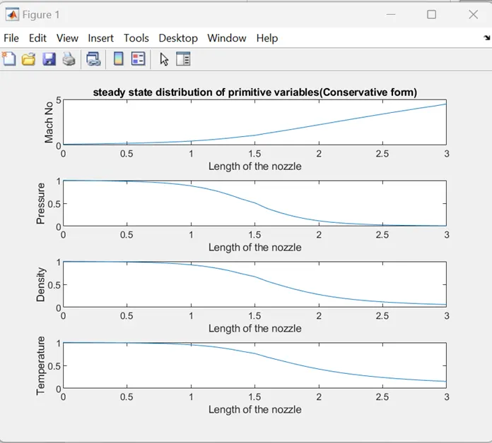
From the plot we can see that Mach number at inlet is subsonic and Mach number at outlet is supersonic. Also Mach number 1 is achieved at the throat. i.e at length 1.5.

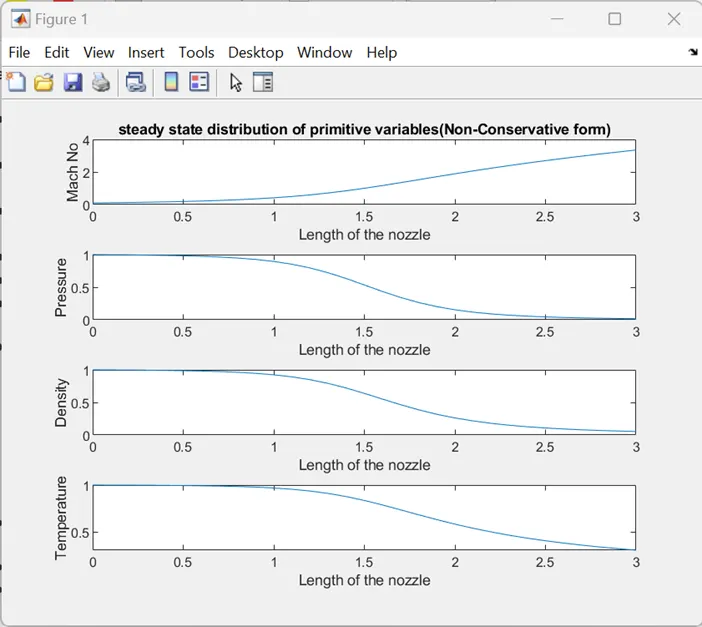
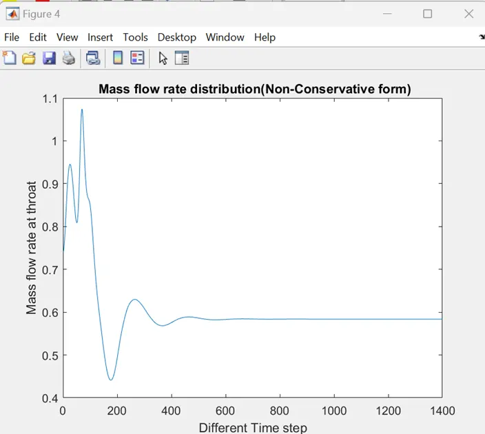
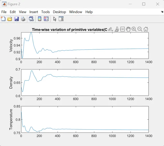
Steady state reached nearly at 500 th time step

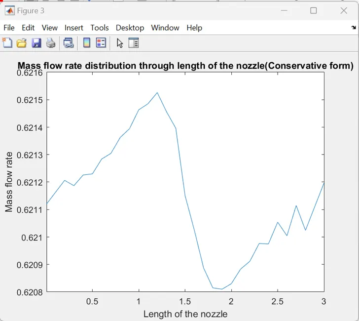
Mass flow rate distribution along the Length of the nozzle

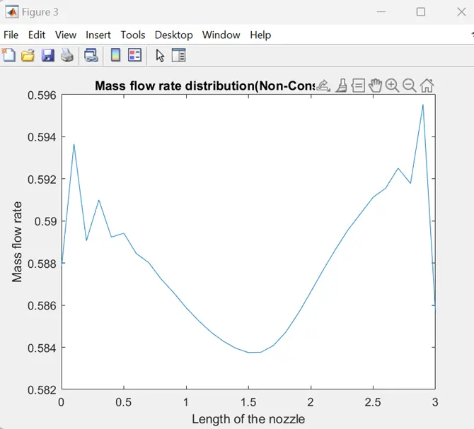
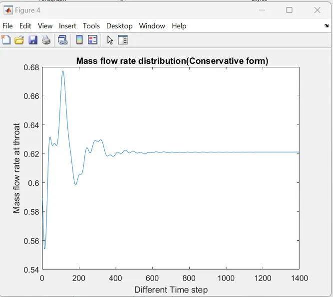
Mass flow rate distribution at throat

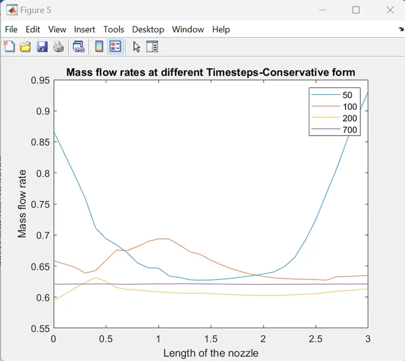
Mass flow rate distribution at different time step

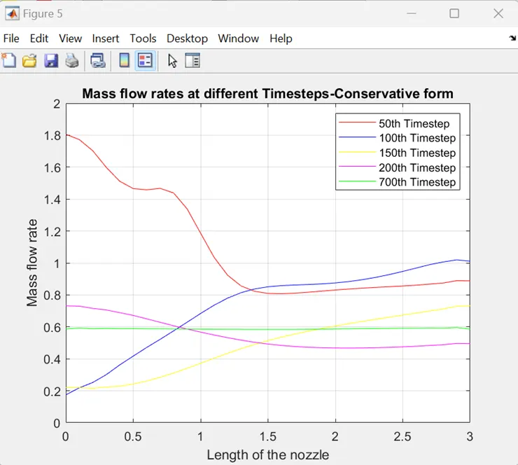
From the above graph we can see that at 700^th time steps, the mass flow distribution is a straight, horizontal line across the graph. This says that the mass flow has converged to a constant, steady-state value throughout the nozzle.

Governing equations for Conservative form

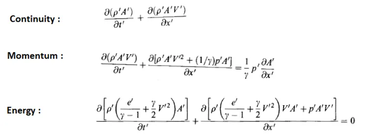
Let us define the elements of the solutions vector U, the flux vector F, and the source term J as follows.

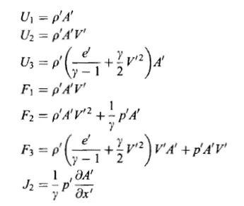
By substituting the above formula in the governing equation, we get

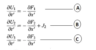
We are now finished with the governing equations for quasi-one-dimensional flow.

The above equations represent the continuity, momentum and energy equations for quasi-one-dimensional flow, in a conservative form. The term U is called the solution vector, to obtain the primitive variables (ρ, V, T, p, etc), we need to decode the elements U₁, U₂ and U₃

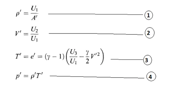
After obtaining U₁, U₂, U₃ at each time step , we immediately calculate the corresponding primitive variables at each time step, ρ’, V’, T’, p’ from equations 1 to 4. These primitive variables would in turn, be used to construct F₁, F₂, F₃ for use in the solution of equation A to C for the next time step and so forth.

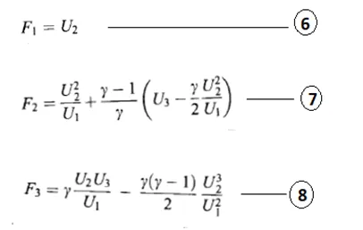
From the above equations we can derive the flux terms in terms of U₁, U₂, U₃ as follows.

The source term J₂ is given by

Equations A to C and flux terms 6 to 8 and source term 9 all are expressed in terms of U1, U2 and U3 only, the primitive variables are not found. This is the pure form of the governing equations in conservative form.

Boundary Conditions

In the subsonic inflow boundary two properties are held fixed and one is allowed to float, and at the supersonic outflow boundary all properties are allowed to float.

We fix ρ’, T’, both equal to 1 and allow V’ to float. Then U1 at grid point i=1 is fixed, independent of time, via U1=ρ’ A’ . That is,

U_1(i=1) = (ρ’A’)_i=1 = A’_i =1 = fixed value

The floating value of V’ at the inflow boundary is calculated at the end of each time step by linearly extrapolating U₂ from the known values at the internal grid points i=2 and 3, that is,

U_2(i=1) = 2 U_2(i=2) – U_2(i=3)

and then obtaining V’ at i=1 from equation 2.

The flow properties at the downstream, supersonic outflow boundary are obtained by linear extrapolation from the two adjacent internal points. If N denotes the grid point at the outflow boundary, then

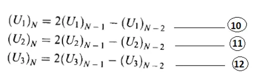
The values of F1, F2 and F3 at grid point i=N are obtained from values of U1, U2 and U3 at i=N using equations 6 to 8.

Initial Conditions

The initial conditions for U1, U2 and U3 were calculated by assuming the following variations of ρ’ and T’

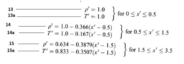
The initial condition for the variation of V’ is synthesized by taking advantage of the fact that one of the dependent variables in our governing equations, namely, U2, is physically the local mass flow; that is U2 = ρ’ A’ V’. Therefore, for the initial conditions only, let us assume a constant mass flow through the nozzle and calculate V’ as

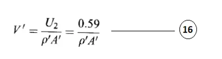
The initial condition for V’ as function of x’ is obtained by substituting the ρ’ variation given by 13, 14 and 15 into equation 16.

Finally the initial conditions for U1, U2, U3 are obtained by substituting the above variations for ρ’, T’ and V’ into the below formals.

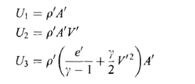
Time step calculation is same as we discussed for non-conservative form.

Conservative form of Quasi-one-dimensional flow

Matlab code

clear all

close all

clc

% conservative form

% inputs

n=31;

x=linspace(0, 3, n);

dx=x(2)-x(1);

gamma=1.4;

% calculate initial profiles

for i=1:length(x)

if x(i)>=0 && x(i)<0.5

rho(i)=1;

t(i)=1;

elseif x(i)>=0.5 && x(i)<1.5

rho(i)=1-0.366*(x(i)-0.5);

t(i)=1-0.167*(x(i)-0.5);

elseif x(i)>=1.5 && x(i)<=3

rho(i)=0.634-0.3879*(x(i)-1.5);

t(i)=0.833-0.3507*(x(i)-1.5);

% area

end

A(i)=1+2.2*(x(i)-1.5).^2; % A=area

end

throat =find(A == 1);

p=rho.*t

v=0.59./(rho.*A);

U1=rho.*A;

U2=rho.*A.*v;

U3=rho.*((t/(gamma-1))+((gamma/2)*v.^2)).*A;

CFL=0.5

dt=min((CFL.*dx)./(v+sqrt(t)));

% outer time loop

for k=1:1400

U1_old= U1;

U2_old= U2;

U3_old= U3;

F1=U2;

F2=(U2.^2./U1)+((gamma-1)/gamma).*(U3-(gamma/2)*(U2.^2./U1));

F3=((gamma.*U2.*U3)./U1)-((gamma.*(gamma-1).*U2.^3)/(2.*U1.^2));

% solution Variable initialization

for i=2:n-1 % predictor loop

J2_p(i)=(1/gamma).*rho(i).*t(i).*((A(i+1)-A(i))./dx);

dU1dt_p(i)=-(F1(i+1)-F1(i))/dx;

dU2dt_p(i)=-(F2(i+1)-F2(i))/dx +J2_p(i);

dU3dt_p(i)=-(F3(i+1)-F3(i))/dx;

% dU1dt_p(i)=(-F1(i+1)-F1(i))/dx;

% dU2dt_p(i)=(-F2(i+1)-F2(i))/dx +J2_p(i);

% dU3dt_p(i)=(-F3(i+1)-F3(i))/dx;

% solution update

U1(i)=U1(i)+dU1dt_p(i).*dt;

U2(i)=U2(i)+dU2dt_p(i).*dt;

U3(i)=U3(i)+dU3dt_p(i).*dt;

end

% decode primitive variables

rho=U1./A;

v=U2./U1;

% update t

t=(gamma-1)*((U3./U1)-(gamma/2)*(v.^2));

% Find the predicted values of F1,F2,F3

F1=U2;

F2=(U2.^2./U1)+((gamma-1)/gamma).*(U3-(gamma/2)*(U2.^2./U1));

F3=((gamma.*U2.*U3)./U1)-((gamma.*(gamma-1).*U2.^3)/(2.*U1.^2));

for i=2:n-1

% Corrector Step

J2_c(i)=(1/gamma)*rho(i)*t(i)*((A(i)-A(i-1))/dx);

dU1dt_c(i)=-(F1(i)-F1(i-1))/dx;

dU2dt_c(i)=-(F2(i)-F2(i-1))/dx + J2_c(i);

dU3dt_c(i)=-(F3(i)-F3(i-1))/dx;

% dU1dt_c(i)=(-F1(i)-F1(i-1))/dx;

% dU2dt_c(i)=(-F2(i)-F2(i-1))/dx + J2_c(i);

% dU3dt_c(i)=(-F3(i)-F3(i-1))/dx;

end

% computing the average

dU1_dt=0.5*(dU1dt_p+dU1dt_c);

dU2_dt=0.5*(dU2dt_p+dU2dt_c);

dU3_dt=0.5*(dU3dt_p+dU3dt_c);

% final solution update

for j=2:n-1

U1(j)=U1_old(j)+dU1_dt(j).*dt;

U2(j)=U2_old(j)+dU2_dt(j).*dt;

U3(j)=U3_old(j)+dU3_dt(j).*dt;

end

% update the boundary conditions

%inlet

U1(1)=A(1).*rho(1);

U2(1)=2*U2(2)-U2(3);

U3(1)=U1(1)*((t(1)/(gamma-1))+(gamma/2)*(v(1)^2));

%outlet

U1(n)=2*U1(n-1)-U1(n-2);

U2(n)=2*U2(n-1)-U2(n-2);

U3(n)=2*U3(n-1)-U3(n-2);

% decoding the corrected values of primitive variables

rho=U1./A;

v=U2./U1;

t=(gamma-1)*((U3./U1)-(gamma/2)*(v.^2));

p=rho.*t;

mass_flow_rate=rho.*A.*v;

% mass_flow_rate(k,:)= rho.*A.*v;

mach_no=v./(t.^0.5);

rho_throat(k)= rho(throat);

v_throat(k)=v(throat);

t_throat(k)=t(throat);

mass_flow_rate_throat(k)=mass_flow_rate(throat);

mach_no_throat(k)=mach_no(throat);

if k==50

m_50=mass_flow_rate;

end

if k==100

m_100=mass_flow_rate;

end

if k==200

m_200=mass_flow_rate;

end

if k==700

m_700=mass_flow_rate;

end

if k==1400

m_1400=mass_flow_rate;

end

if k==800

m_800=mass_flow_rate;

end

if k==1000

m_1000=mass_flow_rate;

end

end

% steady state distribution of primitive variables

figure(1)

subplot(4,1,1)

plot(x, mach_no)

xlabel('Length of the nozzle')

ylabel('Mach No')

title('steady state distribution of primitive variables(Conservative form)')

subplot(4,1,2)

plot(x, p)

xlabel('Length of the nozzle')

ylabel('Pressure')

subplot(4,1,3)

plot(x, rho)

xlabel('Length of the nozzle')

ylabel('Density')

subplot(4,1,4)

plot(x, t)

xlabel('Length of the nozzle')

ylabel('Temperature')

% time-wise variation of primitive variables

figure(2)

subplot(3,1,1)

plot(1:1400, v_throat)

ylabel('Velocity')

title('Time-wise variation of primitive variables(Conservative form)')

subplot(3,1,2)

plot(1:1400, rho_throat)

ylabel('Density')

subplot(3,1,3)

plot(1:1400, t_throat)

ylabel('Temperature')

figure(3)

plot(x, m_1400)

xlabel('Length of the nozzle')

ylabel('Mass flow rate')

title('Mass flow rate distribution through length of the nozzle(Conservative form)')

figure(4)

plot(1:1400, mass_flow_rate_throat)

xlabel('Different Time step')

ylabel('Mass flow rate at throat')

title(' Mass flow rate distribution(Conservative form)')

figure(5)

plot(x,m_50)

hold on

plot(x,m_100)

hold on

plot(x,m_200)

hold on

plot(x,m_700)

title('Mass flow rates at different Timesteps-Conservative form')

xlabel('Length of the nozzle')

ylabel('Mass flow rate')

legend({'50', '100','200', '700'})

Output

Steady-state distribution of primitive variables

Time-wise variation of primitive Variables

Mass flow rate distribution through length of the nozzle

Mass flow rate distribution along the throat at different time step

Mass flow rate along the length of the nozzle at different time step

Grid independence Test

Non-conservative form
	grid point =31	grid point= 61
rho	0.05286653	0.052653304
t	0.308284093	0.307897999
p	0.01629791	0.016211847

Conservative form
	grid point =31	grid point= 61
rho	0.059854078	0.067915704
t	0.150854429	0.234993008
p	0.009029253	0.015959716

For Non-conservative form the solution remains same for grid point 31 and 61. Hence the solution is grid independent.

For conservative form the solution is not same and the solution blows up for grid points 61.

Conclusion

In summary, we cannot establish a clear superiority of the conservation form of the governing equations over the non-conservation form.

Comparing the amount of calculational effort to achieve a solution, we note that the solution of the conservation form requires more work.