Week 5.1 - Mid term project - Solving the steady and unsteady 2D heat conduction problem

Solving the Steady and unsteady 2D heat conduction problem

Aim:

Solving the steady state and transient state 2D heat conduction problem using iterative techniques such as Jacobi, Gauss-seidel and Successive over-relaxation.

Problem Statement

• Assuming the computational area as Square.
• Assume nx=ny=10, which is number of nodes in x and y direction.
• Boundary Conditions are given below.

Left Temperature = 400 K

Right Temperature = 800 K

Top Temperature = 600 K

Bottom Temperature = 900 K

• Assuming the Temperature 300 K for inner nodes.
• Steady state 2D Heat conduction equation is solved by iterative techniques such as Jacobi, Gauss-seidel and Successive over relaxation.(Implicit method)
• Transient 2D Heat conduction equation is solved through Explicit and Implicit method.
• Comparing the number of iterations required in explicit and implicit method to solve steady and transient heat conduction equation.

Theory

Steady state 2D Heat conduction equation

For two dimensional steady state, with no heat generation, the Laplace equation can be given by

`(del^2T)/(dely^2)+(del^2T)/(dely^2)=0`

Jacobi Method

To solve the problem implicitly using Jacobi Method,

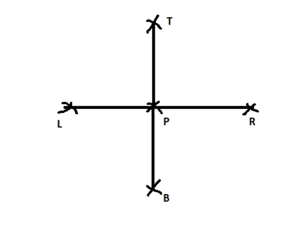
`T_P=(1/K)((T_L+T_R)/(Deltax^2))+(1/K)((T_T+T_B)/(Deltay^2))`

Where T_P = Temperature at a mid point

T_L= Temperature of Left Boundary

T_R= Temperature of Right Boundary

T_T= Temperature of Top Boundary

T_B = Temperature of Bottom Boundary

Jacobian method or Jacobi method is one the iterative methods for approximating the solution of a system of n linear equations in n variables. The Jacobi iterative method is considered as an iterative algorithm which is used for determining the solutions for the system of linear equations in numerical linear algebra, which is diagonally dominant. In this method, an approximate value is filled in for each diagonal element.

 Until it converges, the process is iterated. This algorithm was first called the Jacobi transformation process of matrix diagonalization. Jacobi Method is also known as the simultaneous displacement method.

Let us consider the following system of equation

`a_1 X_1+b_1X_2+c_1X_3= d_1`

`a_2 X_1+b_2X_2+c_2X_3= d_2`

`a_3 X_1+b_3X_2+c_3X_3= d_3`

`AX=B`

`[[a_1 b_1 c_1],[a_2 b_2 c_2],[a_3 b_3 c_3]][[X_1], [X_2], [X_3]]=[[d_1],[d_2],[d_3]]`

When calculating ‘X_1’, ‘X_2’. ‘X_3’ values we use old values for each iteration in Jacobi method.

`X_1^(k+1)=d_1-(b_1X_2^(k))-(c_1X_3^k)`

`X_2^(k+1)=d_2-(a_2X_1^(k))-(c_2X_3^k)`

 `X_3^(k+1)=d_3-(a_3X_1^(k))-(b_3X_3^k)`

Gauss-Seidel

In Jacobi method the value of the variables is not modified until next iteration, whereas in Gauss-Seidel method the value of the variables are modified as soon as new value is evaluated. For instance, in Jacobi method the value of x_i^(k) is not modified until the (k + 1)th iteration but in Gauss-Seidel method the value of x_i^(k) changes in in kth iteration only.

`X_1^(k+1)=d_1-(b_1X_2^(k))-(c_1X_3^k)`

`X_2^(k+1)=d_2-(a_2X_1^(k+1))-(c_2X_3^k)`

`X_3^(k+1)=d_3-(a_3X_1^(k+1))-(b_3X_2^(k+1))`

Successive Over-relaxation

The method of successive over-relaxation (SOR) is a variant of the Gauss–Seidel method for solving a linear system of equations, resulting in faster convergence. A similar method can be used for any slowly converging iterative process.

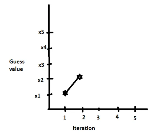
`X_2=X_1+alpha[(x_2-x_1)/(2-1)(1)]`

`[(x_2-x_1)/(2-1)]` is a slope and is brought by Jacobi or Gauss seidel method.

`alpha` - is Scaling factor, when `alpha`>1, then the iterative solver is over tuned and is called over relaxation.

When `alpha`<1, then the iterative solver is under tuned and is called as under relaxation.

Matlab code for steady state 2D heat conduction equation using iterative Techniques

clear all

close all

clc

% solving steady state 2D heat conduction Equation Implicitly

% input Parameters

% Defining Geometry

nx=10;

ny=10

x=linspace(0, 1, nx);

y=linspace(0, 1, ny);

dx=x(2)-x(1);

dy=y(2)-y(1);

% Defining Temperature

T=300*ones(nx, ny);

T_T=600;

T_B=900;

T_L=400;

T_R=800;

% Defining corner Temperature

T(1,1)= (T_T+T_L)/2;

T(1,ny)=(T_T+T_R)/2;

T(nx,1)=(T_L+T_B)/2;

T(nx,ny)=(T_R+T_B)/2;

% Defining the Boundary Temperature

T(2:ny-1,1)=T_L;

T(2:ny-1,nx)=T_R;

T(1, 2:nx-1)=T_T;

T(ny,2:nx-1)=T_B;

% Assigning the initial values to T

T_initial=T;

T_old=T;

% Calculating value of T_P formula

% T_P=(1/K)((T_L+T_R)/dx^2)+(1/K)((T_T+T_B)/dy^2)

K=2*((dx^2+dy^2)/((dx^2)*(dy^2)));

% solving 2D heat conduction equation by Jacobi Method

error=1e9;

tolerence=1e-4;

Jacobi_iteration=1

while error>tolerence

    for i= 2:nx-1

        for j=2:ny-1

            term1=(T_old(i-1,j)+T_old(i+1,j))/(K*dx^2);

            term2=(T_old(i,j-1)+T_old(i,j+1))/(K*dy^2);

            T(i,j)=term1+term2;

        end

    end

    error=max(max(abs(T_old-T)));

    T_old=T;

    Jacobi_iteration=Jacobi_iteration+1;

end

% Plotting

figure(1)

contourf(x,y,T)

clabel(contourf(x,y,T))

colorbar

colormap(jet)

set(gca, 'YDIR', 'reverse')

xlabel('X axis');

ylabel('Y axis');

title_text=sprintf('Steady state-Jacobi Iteration(IMPLICIT)= %d', Jacobi_iteration);

title(title_text)

pause(0.03)

%%

% GS Method

% input Parameters

% Defining Geometry

nx=10;

ny=10

x=linspace(0, 1, nx);

y=linspace(0, 1, ny);

dx=x(2)-x(1);

dy=y(2)-y(1);

% Defining Temperature

T=300*ones(nx, ny);

T_T=600;

T_B=900;

T_L=400;

T_R=800;

% Defining corner Temperature

T(1,1)= (T_T+T_L)/2;

T(1,ny)=(T_T+T_R)/2;

T(nx,1)=(T_L+T_B)/2;

T(nx,ny)=(T_R+T_B)/2;

% Defining the Boundary Temperature

T(2:ny-1,1)=T_L;

T(2:ny-1,nx)=T_R;

T(1, 2:nx-1)=T_T;

T(ny,2:nx-1)=T_B;

% Assigning the initial values to T

T_initial=T

T_old=T;

% Calculating value of T_P formula

% T_P=(1/K)((T_L+T_R)/dx^2)+(1/K)((T_T+T_B)/dy^2)

K=2*((dx^2+dy^2)/((dx^2)*(dy^2)));

% solving 2D heat conduction equation by Gauss-seidel iterative

% technique

error=1e9;

tolerence=1e-4;

Gauss_seidel=1

while error>tolerence

    for i= 2:nx-1

        for j=2:ny-1

            term1=(T(i-1,j)+T_old(i+1,j))/(K*dx^2);

            term2=(T(i,j-1)+T_old(i,j+1))/(K*dy^2);

            T(i,j)=term1+term2

        end

    end

    error=max(max(abs(T_old-T)));

    T_old=T;

    Gauss_seidel=Gauss_seidel+1;

end

% Plotting

figure(2)

contourf(x,y,T)

clabel(contourf(x,y,T))

colorbar

colormap(jet)

set(gca, 'YDIR', 'reverse')

xlabel('X axis');

ylabel('Y axis');

title_text=sprintf('Steady state-Gauss seidel iteration(IMPLICIT)= %d',Gauss_seidel);

title(title_text)

pause(0.03)

%%

% SOR Method

% input Parameters

% Defining Geometry

nx=10;

ny=10

x=linspace(0, 1, nx);

y=linspace(0, 1, ny);

dx=x(2)-x(1);

dy=y(2)-y(1);

% Defining Temperature

T=300*ones(nx, ny);

T_T=600;

T_B=900;

T_L=400;

T_R=800;

% Defining corner Temperature

T(1,1)= (T_T+T_L)/2;

T(1,ny)=(T_T+T_R)/2;

T(nx,1)=(T_L+T_B)/2;

T(nx,ny)=(T_R+T_B)/2;

% Defining the Boundary Temperature

T(2:ny-1,1)=T_L;

T(2:ny-1,nx)=T_R;

T(1, 2:nx-1)=T_T;

T(ny,2:nx-1)=T_B;

% Assigning the initial values to T

T_initial=T

T_old=T;

% Calculating value of T_P formula

% T_P=(1/K)((T_L+T_R)/dx^2)+(1/K)((T_T+T_B)/dy^2)

K=2*((dx^2+dy^2)/((dx^2)*(dy^2)));

% solving 2D heat conduction equation by SOR Method

error=1e9;

tolerence=1e-4;

omega=1.2

SOR=1

while error>tolerence

    for i= 2:nx-1

        for j=2:ny-1

            term1=(T(i-1,j)+T_old(i+1,j))/(K*dx^2);

            term2=(T(i,j-1)+T_old(i,j+1))/(K*dy^2);

            T_GS=term1+term2;

            T(i,j)=(1-omega)*T_old(i,j)+omega*T_GS

        end

    end

    error=max(max(abs(T_old-T)));

    T_old=T;

    SOR=SOR+1;

end

% Plotting

figure(3)

contourf(x,y,T)

clabel(contourf(x,y,T))

colorbar

colormap(jet)

set(gca, 'YDIR', 'reverse')

xlabel('X axis');

ylabel('Y axis');

title_text=sprintf('Steady state-SOR(IMPLICIT)= %d',SOR);

title(title_text)

pause(0.03)

%%

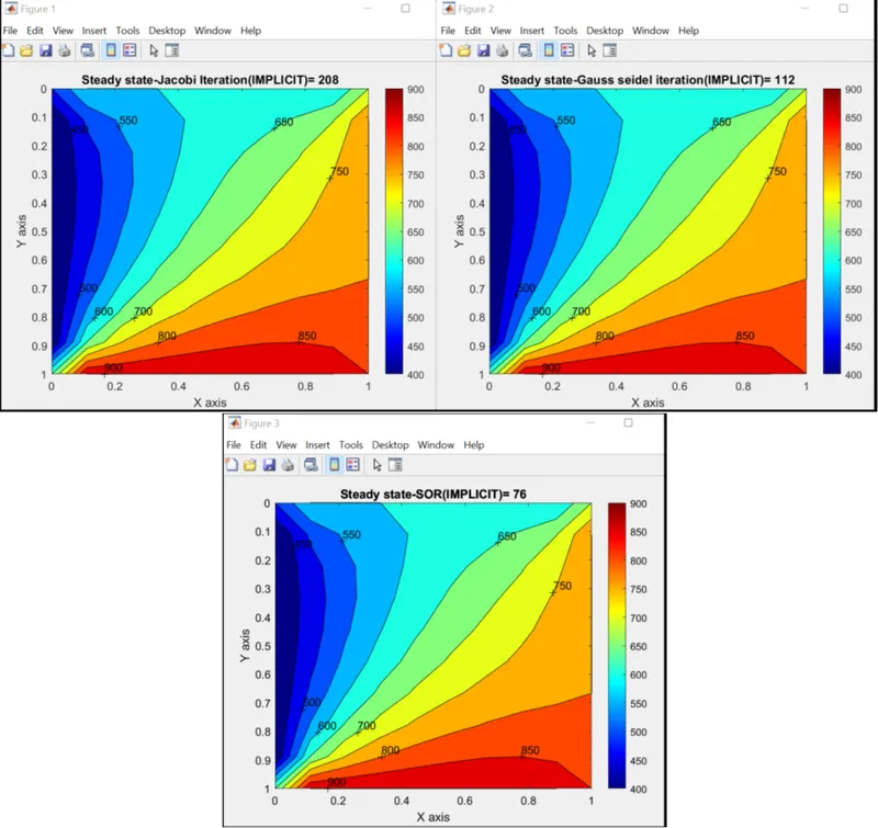
 Result

 

 Transient State 2D heat conduction equation-Solving Explicitly

`(delT)/(delt)=alpha((del^2T)/(delx^2)+(del^2T)/(dely^2))`

`(T_P^(n+1)_T_P^n)/(Deltat)-alpha[(T_L^n-2T_P^n+T_R^n)/(Deltax^2)+(T_T^n-2T_P^n+T_B^n)/(Deltay^2)]=0`

`T_P^(n+1)=T_P^n+K_1(T_L-2T_p+T_R)^n+K_2(T_T-2T_p+T_B)^n`

`K_1= (alphaDeltat)/(Deltax^2)`                             `K_2= (alphaDeltat)/(Deltay^2)`

‘K_1’=CFL No along x direction

‘K_2’CFL No along y direction

Total CFL No should be less than or equal to 5, Otherwise the solution will be unstatble.

So we have assumed dt=0.001 and Total CFL Value kept below 5.

Matlab code for solving 2D Transient heat conduction equation using explicit approach

clear all

close all

clc

% Transient heat conduction equation-solving through explicit method

% input Parameters

% Defining Geometry

nx=10;

ny=10

nt=1400

dt=0.001

x=linspace(0, 1, nx);

y=linspace(0, 1, ny);

dx=x(2)-x(1);

dy=y(2)-y(1);

% Defining Temperature

T=300*ones(nx, ny);

T_T=600;

T_B=900;

T_L=400;

T_R=800;

% Defining corner Temperature

T(1,1)= (T_T+T_L)/2;

T(1,ny)=(T_T+T_R)/2;

T(nx,1)=(T_L+T_B)/2;

T(nx,ny)=(T_R+T_B)/2;

% Defining the Boundary Temperature

T(2:ny-1,1)=T_L;

T(2:ny-1,nx)=T_R;

T(1, 2:nx-1)=T_T;

T(ny,2:nx-1)=T_B;

% Assigning the initial values to T

T_initial=T;

T_old=T;

alpha=1.4;

k1=alpha*(dt/dx^2);

k2=alpha*(dt/dy^2);

Total_CFL=k1+k2;

tolerence=1e-4

error=1e9

unsteady_explicit=1

for nt=1:1400

    for i= 2:nx-1

        for j=2:ny-1

            term1=T_old(i,j);

            term2=k1*(T_old(i-1,j)-2*T_old(i,j)+T_old(i+1,j));

            term3=k2*(T_old(i,j+1)-2*T_old(i,j)+T_old(i,j-1));

            T(i,j)=term1+term2+term3;

        end

    end

    T_old=T;

    unsteady_explicit=unsteady_explicit+1;

end

% Plotting

figure(1)

contourf(x,y,T)

clabel(contourf(x,y,T))

colorbar

colormap(jet)

set(gca, 'YDIR', 'reverse')

xlabel('X axis');

ylabel('Y axis');

title_text=sprintf('Unsteady Explicit iteration= %d',unsteady_explicit);

title(title_text)

pause(0.03)

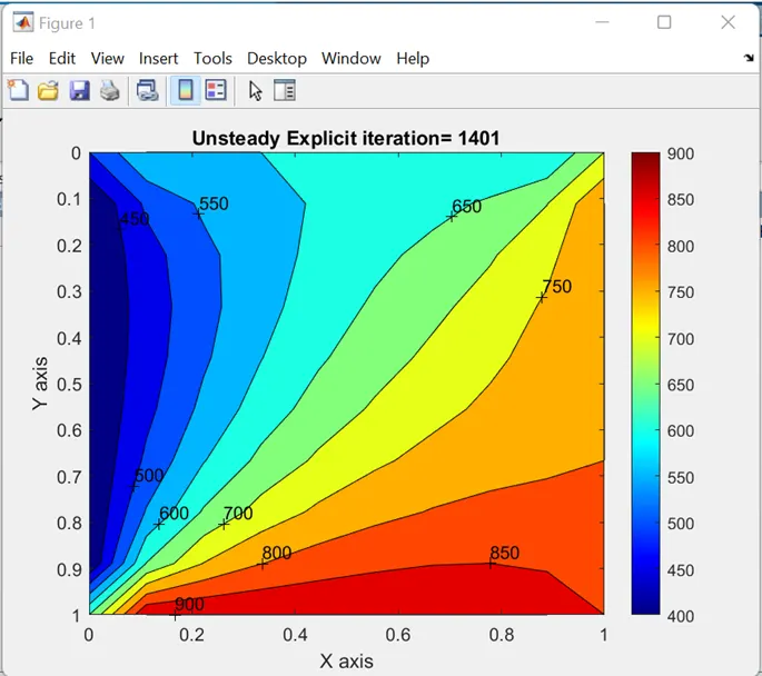
 Result

Matlab code for solving 2D Transient heat conduction equation using implicit approach

clear all

close all

clc

% Solving transient heat conduction using iterative Technique(Implicit)

% input Parameters

% Defining Geometry

nx=10;

ny=10

dt=0.01

x=linspace(0, 1, nx);

y=linspace(0, 1, ny);

dx=x(2)-x(1);

dy=y(2)-y(1);

% Defining Temperature

T=300*ones(nx, ny);

T_T=600;

T_B=900;

T_L=400;

T_R=800;

% Defining corner Temperature

T(1,1)= (T_T+T_L)/2;

T(1,ny)=(T_T+T_R)/2;

T(nx,1)=(T_L+T_B)/2;

T(nx,ny)=(T_R+T_B)/2;

% Defining the Boundary Temperature

T(2:ny-1,1)=T_L;

T(2:ny-1,nx)=T_R;

T(1, 2:nx-1)=T_T;

T(ny,2:nx-1)=T_B;

% Assigning the initial values to T

T_initial=T

T_pre_dt=T;

T_old=T;

% Calculating value of T_P formula

alpha=1.4;

k1=alpha*(dt/dx^2);

k2=alpha*(dt/dy^2);

% solving 2D heat conduction equation by Jacobi Method

tolerence=1e-4;

Jacobi_iteration=1

for k=1:1400

    error=1e9;

    while error>tolerence

        for i= 2:nx-1

            for j=2:ny-1

                term1=1/(1+2*k1+2*k2);

                term2=k1*term1;

                term3=k2*term1;

                H=T_old(i-1,j)+T_old(i+1,j);

                V=T_old(i,j-1)+T_old(i,j+1);

                T(i,j)=term1*T_pre_dt(i,j)+term2*H+term3*V;

            end

        end

        error=max(max(abs(T_old-T)));

        T_old=T;

        Jacobi_iteration=Jacobi_iteration+1;

    end

    T_pre_dt=T;

end

% Plotting

figure(1)

contourf(x,y,T)

clabel(contourf(x,y,T))

colorbar

colormap(jet)

set(gca, 'YDIR', 'reverse')

xlabel('X axis');

ylabel('Y axis');

title_text=sprintf('Unsteady-Jacobi Iteration(IMPLICIT)= %d', Jacobi_iteration);

title(title_text)

pause(0.03)

%%

% input Parameters

% Defining Geometry

nx=10;

ny=10

dt=0.01

x=linspace(0, 1, nx);

y=linspace(0, 1, ny);

dx=x(2)-x(1);

dy=y(2)-y(1);

% Defining Temperature

T=300*ones(nx, ny);

T_T=600;

T_B=900;

T_L=400;

T_R=800;

% Defining corner Temperature

T(1,1)= (T_T+T_L)/2;

T(1,ny)=(T_T+T_R)/2;

T(nx,1)=(T_L+T_B)/2;

T(nx,ny)=(T_R+T_B)/2;

% Defining the Boundary Temperature

T(2:ny-1,1)=T_L;

T(2:ny-1,nx)=T_R;

T(1, 2:nx-1)=T_T;

T(ny,2:nx-1)=T_B;

% Assigning the initial values to T

T_initial=T

T_pre_dt=T;

T_old=T;

% Calculating value of T_P formula

alpha=1.4;

k1=alpha*(dt/dx^2);

k2=alpha*(dt/dy^2);% solving 2D heat conduction equation by Gauss seidel Method

tolerence=1e-4;

% Calculating 2D heat conduction equation by Gauss-seidel

GS=1

for k=1:1400

    error=1e9;

    while error>tolerence

        for i= 2:nx-1

            for j=2:ny-1

                term1=1/(1+2*k1+2*k2);

                term2=k1*term1;

                term3=k2*term1;

                H=T(i-1,j)+T_old(i+1,j);

                V=T(i,j-1)+T_old(i,j+1);

                T(i,j)=term1*T_pre_dt(i,j)+term2*H+term3*V;

            end

        end

        error=max(max(abs(T_old-T)));

        T_old=T;

        GS=GS+1;

    end

    T_pre_dt=T;

end

% Plotting

figure(2)

contourf(x,y,T)

clabel(contourf(x,y,T))

colorbar

colormap(jet)

set(gca, 'YDIR', 'reverse')

xlabel('X axis');

ylabel('Y axis');

title_text=sprintf('Unsteady-Gauss seidel iteration(IMPLICIT)= %d',GS);

title(title_text)

pause(0.03)

%%

% input Parameters

% Defining Geometry

nx=10;

ny=10

dt=0.01

x=linspace(0, 1, nx);

y=linspace(0, 1, ny);

dx=x(2)-x(1);

dy=y(2)-y(1);

% Defining Temperature

T=300*ones(nx, ny);

T_T=600;

T_B=900;

T_L=400;

T_R=800;

% Defining corner Temperature

T(1,1)= (T_T+T_L)/2;

T(1,ny)=(T_T+T_R)/2;

T(nx,1)=(T_L+T_B)/2;

T(nx,ny)=(T_R+T_B)/2;

% Defining the Boundary Temperature

T(2:ny-1,1)=T_L;

T(2:ny-1,nx)=T_R;

T(1, 2:nx-1)=T_T;

T(ny,2:nx-1)=T_B;

% Assigning the initial values to T

T_initial=T

T_pre_dt=T;

T_old=T;

% Calculating value of T_P formula

alpha=1.4;

k1=alpha*(dt/dx^2);

k2=alpha*(dt/dy^2);

omega=1.2;

% solving 2D heat conduction equation by SOR method

tolerence=1e-4;

% Calculating 2D heat conduction equation by SOR

SOR=1

for k=1:1400

    error=1e9;

    while error>tolerence

        for i= 2:nx-1

            for j=2:ny-1

                term1=1/(1+2*k1+2*k2);

                term2=k1*term1;

                term3=k2*term1;

                H=T(i-1,j)+T_old(i+1,j);

                V=T(i,j-1)+T_old(i,j+1);

                L=term1*T_pre_dt(i,j)+term2*H+term3*V;

                T(i,j)=(1-omega)*T_old(i,j)+omega*L

            end

        end

        error=max(max(abs(T_old-T)));

        T_old=T;

        SOR=SOR+1;

    end

    T_pre_dt=T;

end

% Plotting

figure(3)

contourf(x,y,T)

clabel(contourf(x,y,T))

colorbar

colormap(jet)

set(gca, 'YDIR', 'reverse')

xlabel('X axis');

ylabel('Y axis');

title_text=sprintf('Unsteady-SOR Iteration(IMPLICIT)= %d',SOR);

title(title_text)

pause(0.03)

 

Result

 

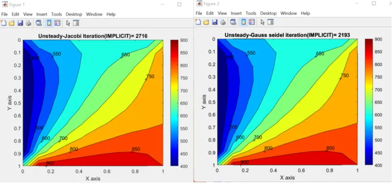
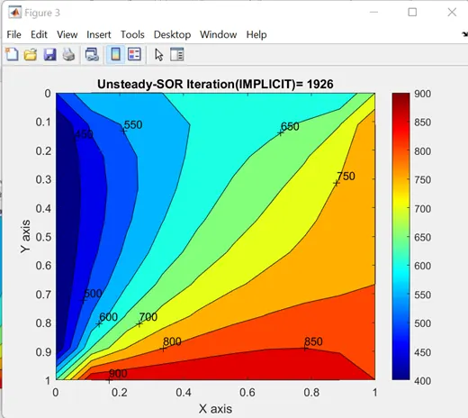
 Conclusion

	No. of Iterations taken to solve the problem
	Jacobi	Gauss-seidel	SOR
Steady State-Implicit	208	112	76
Transient State-Implicit	2716	2193	1926
Transient State-Explicit	1401

 From ablove table, we can say that successive over relaxation takes less number of iteration comparing with Jacobi and Gauss-seidel method in both steady and unsteady problem. In addition to that Transient problem take more iteration than steady state problem.

Following is the order of iterative techniques based on number of iterations.

Jacobi > Gauss-seidel > Successive Over Relaxaion