Week 3.5 - Deriving 4th order approximation of a 2nd order derivative using Taylor Table method

Deriving 4^th order approximation of a 2^nd order derivative using Taylor Table method

Aim:

1. Deriving the following 4^th order approximations of the 2^nd-order derivative and prove that the skewed schemes are 4^th order accurate.

• Central Difference
• Skewed right-sided difference
• Skewed left-sided difference

2. Also writing a program in Matlab to evaluate the second-order derivative of the analytical function exp(x)*cos(x) and compare it with the 3 numerical approximations that we have derived.
3. Plotting a graph that compares the absolute error between the above-mentioned schemes.

Central Difference Approximation:

Number of nodes = P + Q – 1

P – Order of Derivative = 2

Q – Order of Approximation = 4

Number of nodes = 5

`Deltax^2 ((del^2u)/(delx^2))=af(i-2)+bf(i-1)+cf(i)+df(i+1)+ef(i+2)` ------------(A)

`af(i-2)=af(i)-(af'(i)(2Deltax))/(1!)+(af ''(i)(2Deltax)^2)/(2!)-(af'''(i)(2Deltax)^3)/(3!)+(af''''(i)(2Deltax)^4)/(4!)-(af'''''(i)(2Deltax)^5)/(5!)`

`bf(i-1)=bf(i)-(bf'(i)(Deltax))/(1!)+(bf ''(i)(Deltax)^2)/(2!)-(bf'''(i)(Deltax)^3)/(3!)+(bf''''(i)(Deltax)^4)/(4!)-(bf'''''(i)(Deltax)^5)/(5!)`

`cf(i)= cf(i)`

`df(i+1)=df(i)+(df'(i)(Deltax))/(1!)+(df ''(i)(Deltax)^2)/(2!)+(df'''(i)(Deltax)^3)/(3!)+(df''''(i)(Deltax)^4)/(4!)+(df'''''(i)(Deltax)^5)/(5!)`

`ef(i+2)=ef(i)+(ef'(i)(2Deltax))/(1!)+(ef ''(i)(2Deltax)^2)/(2!)+(ef'''(i)(2Deltax)^3)/(3!)+(ef''''(i)(2Deltax)^4)/(4!)+(ef'''''(i)(2Deltax)^5)/(5!)`

Taylor's Table

`Deltax^2(del^2u)/(delx^2)`	`f(i)`	`f'(i)Deltax`	`f''(i)Deltax^2`	`f'''(i)Deltax^3`	`f''''(i)Deltax^4`	`f'''''(i)Deltax^5`	`f''''''(i)Deltax^6`
af(i-2)	a	-2a	4a/2	-8a/6	16a/24	-32a/120	64a/720
bf(i-1)	b	-b	b/2	-b/6	b/24	-b/120	b/720
cf(i)	c	0	0	0	0	0	0
df(i+1)	d	d	d/2	d/6	d/24	d/120	d/720
Ef(i+2)	e	2e	4e/2	8e/6	16e/24	32e/120	64e/720

a+b+c+d+e = 0 ---------------(1)

-2a-b+0+d+2e = 0--------------------(2)

(4a/2)+(b/2)+0+(d/2)+(4e/2) = 1 -------------------------(3)

(-8a/6)-(b/6)+0+(d/6)+(8e/6) = 0 ----------------------(4)

(16a/24)+(b/24)+0+(d/24)+(16e/24) = 0-----------------(5)

AX= B

`[[1,1,1,1,1],[-2,-1,0,1,2],[4,1,0,1,4],[-8,-1,0,1,8],[16,1,0,1,16]][[a],[b],[c],[d],[e]]=[[0],[0],[2],[0],[0]]`

X=A^-1 B

a = -0.0833

b = 1.3333

c = -2.5

d = 1.3333

e = -0.0833

`(a+b+c+d+e)f(i)+(-2a-b+d+2e)f'(i)Deltax+((4a)/2+b/2+d/2+(4e)/2)f''(i)Deltax^2+((-8a)/6-b/6+d/6+(8e)/6)f'''(i)Deltax^3+((16a)/24+b/24+d/24+(16e)/24)f''''(i)Deltax^4+((-32a)/120-b/120+d/120+(32e)/120)f'''''(i)Deltax^5+((64a)/720+b/720+d/720+(64e)/720)f''''''(i)Deltax^6` ---(6)

Substituting the values in Equation 6, we get

`(del^2u)/(delx^2)=(1/(Deltax^2))[((4a)/2+b/2+d/2+(4e)/2)f''(i)Deltax^2+((64a)/720+b/720+d/720+(64e)/720)f''''(i)Deltax^6]`

`(del^2u)/(delx^2)=((4a)/2+b/2+d/2+(4e)/2)f''(i)+((64a)/720+b/720+d/720+(64e)/720)f''''''(i)Deltax^4`

In the above equation `Deltax^4` denotes the truncation error.

As the order of truncation error is 4, the above derived 2^nd order derivative is equation of 4^th order approximation.

After substituting the values in equation A, we get 4^th order approximation of 2^nd order derivative.

`(del^2u)/(delx^2)=-0.0833f(i-2)+1.3333f(i-1)-2.5f(i)+1.3333f(i+1)-0.0833f(i+2)`

Skewed Right sided Difference

Number of nodes = P + Q

P – Order of Derivative = 2

Q – Order of Approximation = 4

Number of nodes = 6

`Deltax^2 ((del^2u)/(delx^2))=af(i)+bf(i+1)+cf(i+2)+df(i+3)+ef(i+4)+gf(i+5)`

Expanding the Taylor series for each term, we get the coefficients as follows,

Taylor's Table

`Deltax^2(del^2u)/(delx^2)`	`f(i)`	`f'(i)Deltax`	`f''(i)Deltax^2`	`f'''(i)Deltax^3`	`f''''(i)Deltax^4`	`f'''''(i)Deltax^5`	`f''''''(i)Deltax^6`
f(i)	a	0	0	0	0	0	0
f(i+1)	b	b	b/2	b/6	b/24	b/120	b/720
f(i+2)	c	2c	4c/2	8c/6	16c/24	32c/120	64c/720
f(i+3)	d	3d	9d/2	27d/6	81d/24	243d/120	729d/720
f(i+4)	e	4e	16e/2	64e/6	256e/24	1024e/120	4096e/720
f(i+5)	g	5g	25g/2	125g/6	625g/24	3125g/120	15625g/720

`[[1,1,1,1,1,1],[0,1,2,3,4,5],[0,1,4,9,16,25],[0,1,8,27,64,125],[0,1,16,81,256,625],[0,1,32,243,1024,3125]][[a],[b],[c],[d],[e],[g]]=[[0],[0],[2],[0],[0],[0]]`

a=3.7500

b=-12.8333

c=17.8333

d =-13

e =5.0833

f = -0.8333

`(del^2u)/(delx^2)=3.75f(i)-12.8333f(i+1)+17.8333f(i+2)-13f(i+3)+5.0833f(i+4)-0.8333f(i+5)`

Skewed Left sided difference

`Deltax^2 ((del^2u)/(delx^2))=af(i-5)+bf(i-4)+cf(i-3)+df(i-2)+ef(i-1)+gf(i)`

Taylor's Table

`Deltax^2(del^2u)/(delx^2)`	`f(i)`	`f'(i)Deltax`	`f''(i)Deltax^2`	`f'''(i)Deltax^3`	`f''''(i)Deltax^4`	`f'''''(i)Deltax^5`	`f''''''(i)Deltax^6`
f(i-5)	a	-5a	25a/2	-125a/6	625a/24	-3125a/120	15625a/720
f(i-4)	b	-4b	16b/2	-64b/6	256b/24	-1024b/120	4096b/720
f(i-3)	c	-3c	9c/2	-27c/6	81c/24	-243c/120	729c/720
f(i-2)	d	-2d	4d/2	-8d/6	16d/24	-32d/120	64d/720
f(i-1)	e	-e	e/2	-e/2	e/24	-e/120	e/720
f(i)	g	0	0	0	0	0	0

`[[1,1,1,1,1,1],[-5,-4,-3,-2,-1,0],[25,16,9,4,1,0],[-125,-64,-27,-8,-1,0],[625,256,81,16,1,0],[-3125,-1024,-243,-32,-1,0]][[a],[b],[c],[d],[e],[g]]=[[0],[0],[2],[0],[0],[0]]`

a= -0.8333

b=5.0833

c=-13

d=17.8333

e=-12.8333

g= 3.75

`(del^2u)/(delx^2)=-0.8333f(i-5)+5.0833f(i-4)-13f(i-3)+17.8333f(i-2)-12.8333f(i-1)+3.75f(i)`

Matlab code

Function code

Central Difference Approximation

function[error]=central_difference_approximation(x, dx)

% Analytical function = exp(x)*cos(x)

% Second_order_analytical_derivative= -2*exp(x)*cox(x)

Analytical_derivative= -2*exp(x)*sin(x)

% central_differencing=(-0.0833f(i-2)+1.3333f(i-1)-2.5f(i)+1.3333f(i+1)-0.0833f(i+2))/dx^2;

a= -(5/60)*(exp(x-(2*dx))*cos(x-(2*dx)))

b= (4/3)*(exp(x-dx)*cos(x-dx))

c=-(5/2)*(exp(x)*cos(x))

d=(4/3)*(exp(x+dx)*cos(x+dx))

e=-(5/60)*(exp(x+(2*dx))*cos(x+(2*dx)))

central_differencing=(a+b+c+d+e)/dx^2

error=abs(central_differencing-Analytical_derivative)

Skewed right sided approximation

function [error ]=skewed_right_sided_approximation(x, dx)

% Analytical function = exp(x)*cos(x)

% Second_order_analytical_derivative= -2*exp(x)*cox(x)

Analytical_derivative= -2*exp(x)*sin(x)

% skewed_right_sided_differencing=(3.75f(i)-12.8333f(i+1)+17.8333f(i+2)-13f(i+3)+5.0833f(i+4)-0.8333f(i+5))/dx^2;

a=(15/4)*(exp(x)*cos(x))

b=-(77/6)*(exp(x+dx)*cos(x+dx))

c=(107/6)*(exp(x+(2*dx))*cos(x+(2*dx)))

d=-13*(exp(x+(3*dx))*cos(x+(3*dx)))

e=(61/12)*(exp(x+(4*dx))*cos(x+(4*dx)))

f=-(5/6)*(exp(x+(5*dx))*cos(x+(5*dx)))

skewed_right_sided_differencing=(a+b+c+d+e+f)/dx^2

error=abs(skewed_right_sided_differencing-Analytical_derivative)

Skewed left sided approximation

function [error] =skewed_left_sided_approximation(x, dx)

% Analytical function = exp(x)*cos(x)

% Second_order_analytical_derivative= -2*exp(x)*cox(x)

Analytical_derivative= -2*exp(x)*sin(x)

% skewed_right_sided_approximation=(-0.8333f(i-5)+5.0833f(i-4)-13f(i-3)+17.8333f(i-2)-12.8333(i-1)+3.75f(i))/dx^2;

%skewed_right_sided_approximation=af(i)+bf(i-1)+cf(i-2)+df(i-3)+ef(i-4)+gf(i-5)

a=-(5/6)*(exp(x-(5*dx))*cos(x-(5*dx)))

b= (61/12)*(exp(x-(4*dx))*cos(x-(4*dx)))

c=-13*(exp(x-(3*dx))*cos(x-(3*dx)))

d=(107/6)*(exp(x-(2*dx))*cos(x-(2*dx)))

e=-(77/6)*(exp(x-dx)*cos(x-dx))

f=(15/4)*(exp(x)*cos(x))

central_differencing=(a+b+c+d+e+f)/dx^2

error=abs(central_differencing-Analytical_derivative)

Main code

clear all

close all

clc

x=pi/3;

dx=linspace(pi/300, pi/30, 20);

for i= 1:length(dx)

% calling function

central_differencing_error(i)=central_difference_approximation(x, dx(i));

skewed_right_sided_error(i)=skewed_right_sided_approximation(x, dx(i));

skewed_left_sided_error(i)=skewed_left_sided_approximation(x, dx(i));

end

loglog(dx, central_differencing_error,'b');

hold on

loglog(dx, skewed_right_sided_error, 'r');

hold on

loglog(dx, skewed_left_sided_error, 'g');

xlabel('Grid size(dx)')

ylabel('Truncation Error')

legend('Central difference', 'Skewed right sided', 'Skewed left sided')

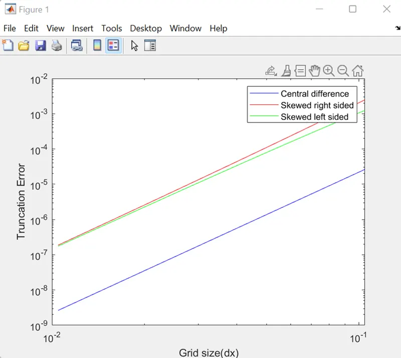
Conclusion:

From the plot we can say that the truncation error of central difference approximation is less compared with skewed schemes.

Because central difference approximation takes information from both sides whereas skewed schemes takes information from one side.

When skewed schemes are useful?

When the system doesn’t have information on both sides, we use information only on one direction and use skewed schemes.