Week 8 - Simulation of a backward facing step in OpenFOAM
Simulation of Backward facing step using OpenFOAM
Aim
Simulating an incompressible-laminar-viscous flow through the backward facing step geometry and performing a transient simulation.
Case 1 - Simulating the flow without using any grading factor (i.e., GF = 1)
Case 2 - Simulating the flow with grading factor of 0.2. The cells should be finer near the walls (includig the step wall).
Backward facing step
Simulation of a backward facing step using the open-source software package OpenFOAM can be used to study the flow dynamics of fluid flow over a step-like obstacle. The backward facing step is a commonly used test case in the study of turbulent flows, as it exhibits complex flow patterns and separation phenomena.
Mesh specification
- Number of cells along the x direction (longer dimension) = 200
- Number of cells along the longer y direction = 20;
Boundary condition specification
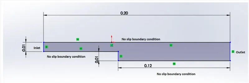
Desired output
- Velocity profile at 0.085 m from the inlet of the geometry for both case studies and compare.
- The reason why Grading/Growth factor is essential for meshing.
Initial Setup
1) To start the simulation, firstly we need to open the Ubuntu terminal, and open Tutorials using the “tut” command.
2) When you give the ls” command, you can see the list of folders inside tutorial folder.
3) Choose the incompressible folder and then icoFoam. Use “cd incompressible” to navigate into the incompressible folder.
4) Then we need to copy the cavity file from icoFoam folder to our run folder. Use cp command to copy.
5) The commands are as follows,
- tut
- ls
- cd incompressible
- ls
- cd icoFoam
- ls
- cp -r cavity $FOAM_RUN/cavity_test
cavity_test folder
We can see the following 3 folders inside Cavity_test folder

- 0
- Constant
- System
0 folder
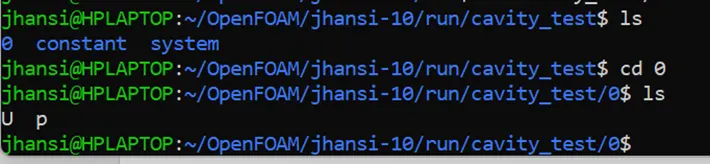
It consists of text file to update initial and boundary condition for velocity (U) and pressure(p)
Constant folder
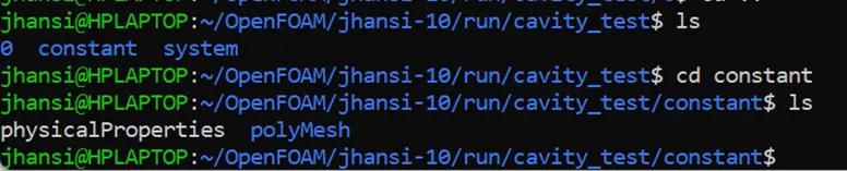
In constant folder we can see text file of physicalProperties and polyMesh folder
System folder

In the system folder we have text files called blockMeshDict, controlDict, fvSchemes, fvSolutions.
- blockMeshDict – To create geometry mesh(block)/ define boundary
- controlDict – To give start time, end time and CFL condition
- fvSchemes – It consists of Navier stokes equation which is required to solve the problem
Changes to be made
For our simulation we need to give initial conditions for velocity and pressure and do some changes in blockMeshDict and controlDict file.
Geometry Creation:
To simulate the backward facing step in OpenFOAM, the first step is to create a computational mesh for the domain of interest.
This can be done by editing the blockMeshDict file. The mesh should be fine enough to capture the details of the flow near the step, but not so fine that it unnecessarily increases the computational cost.
Let us consider creating the geometry using the 5 blocks as shown below.
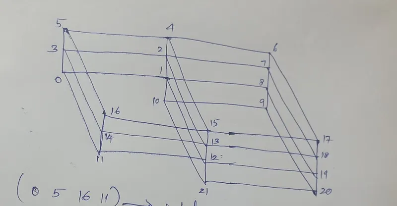
to create the 1st Block for this case,
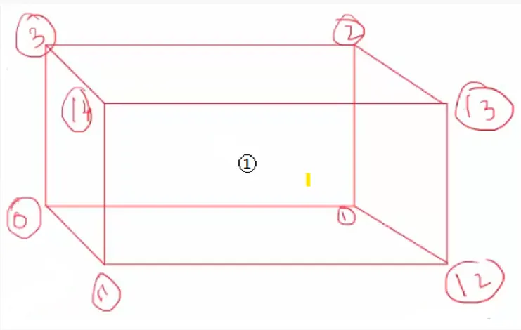
hex (0 1 2 3 11 12 13 14) (1 1 1) simpleGrading (1 1 1)
Similarly proceed by defining the vertices of the other blocks in the Geometry.
To View geometry that you have created, clear out all the entries inside the boundary section of the blockMeshDict file and execute the blockMesh command in the terminal.
Now open paraview and view the geometry that you have created.
Meshing:
Now to mesh the geometry fill in the number of cells in x, y and z direction inside the second parenthesis of the Hex command,
i.e., hex(0 1 2 3 11 12 13 14) (10 10 1) simplegrading(1 1 1).
since this is a 2D problem, increasing the number of cells in the z direction, doesn’t make sense. To view the mesh in paraFoam, select the surface with edges option and view the mesh.
Similarly to refine the mesh near the walls of the geometry, you need to play around with the numbers in the third parenthesis. We leave that for you to figure out, how It can be done.
Boundary Conditions:
Before we run the simulations, we need to specify the initial and boundary conditions.
The given boundary conditions are,
1.Inlet: (Type patch)
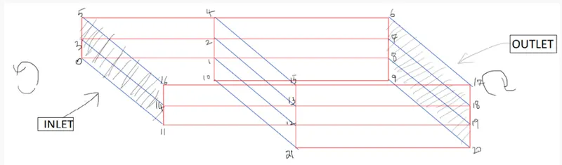
The faces that contribute to inlet boundary are given below. If we are looking at these faces from the outside, the definition of inlet boundary will be in counter-clockwise direction,
(0 11 14 3)
(3 14 16 5)
2.Outlet: (Type patch)
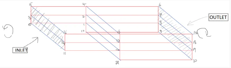
Similarly, we have 3 faces contributing to the outlet boundary condition. Since we are viewing the faces from outside, hence the definition of the outlet boundary will be in counter-clockwise direction,
(9 8 19 20)
(8 7 18 19)
(7 6 17 18)
Now for the other boundary look at the images below and repeat the steps to define the boundaries.
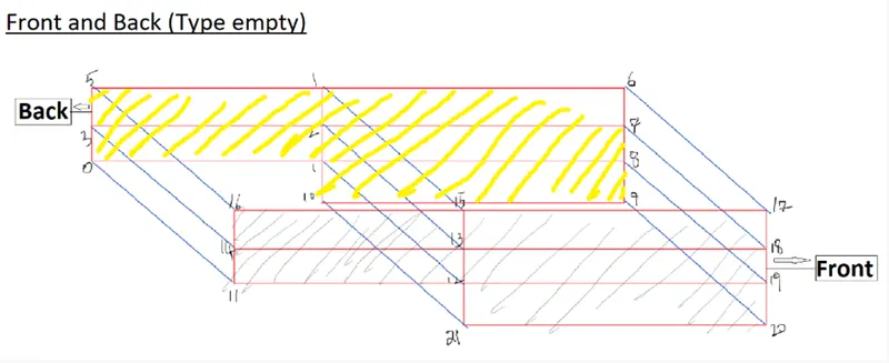
4.No Slip walls: (Type wall)
Top and bottom faces
Top – (16 15 4 5), (15 17 6 4)
Bottom – (11 0 1 12), (21 10 9 20)
Side step – (10 21 12 1)
blockMeshDict File
/*--------------------------------*- C++ -*----------------------------------*\
========= |
\\ / F ield | OpenFOAM: The Open Source CFD Toolbox
\\ / O peration | Website: https://openfoam.org
\\ / A nd | Version: 10
\\/ M anipulation |
\*---------------------------------------------------------------------------*/
FoamFile
{
format ascii;
class dictionary;
object blockMeshDict;
}
// * * * * * * * * * * * * * * * * * * * * * * * * * * * * * * * * * * * * * //
convertToMeters 0.1;
vertices
(
(0 0 0)
(8 0 0)
(8 0.5 0)
(0 0.5 0)
(8 1 0)
(0 1 0)
(20 1 0)
(20 0.5 0)
(20 0 0)
(20 -1 0)
(8 -1 0)
(0 0 0.1)
(8 0 0.1)
(8 0.5 0.1)
(0 0.5 0.1)
(8 1 0.1)
(0 1 0.1)
(20 1 0.1)
(20 0.5 0.1)
(20 0 0.1)
(20 -1 0.1)
(8 -1 0.1)
);
blocks
(
hex (0 1 2 3 11 12 13 14) (80 10 1) simpleGrading (1 1 1)
hex (3 2 4 5 14 13 15 16) (80 10 1) simpleGrading (1 1 1)
hex (2 7 6 4 13 18 17 15) (120 10 1) simpleGrading (1 1 1)
hex (1 8 7 2 12 19 18 13) (120 10 1) simpleGrading (1 1 1)
hex (10 9 8 1 21 20 19 12) (120 20 1) simpleGrading (1 1 1)
);
boundary
(
Inlet
{
type wall;
faces
(
(0 11 14 3)
(3 14 16 5)
);
}
Outlet
{
type wall;
faces
(
(9 8 19 20)
(8 7 18 19)
(7 6 17 18)
);
}
frontAndBack
{
type empty;
faces
(
(11 12 13 14)
(14 13 15 16)
(21 20 19 12)
(12 19 18 13)
(13 18 17 15)
(0 3 2 1)
(3 5 4 2)
(2 4 6 7)
(1 2 7 8)
(10 1 8 9)
);
}
fixedWalls
{
type Wall;
faces
(
(5 16 15 4)
(0 1 12 11)
(4 15 17 6)
(10 9 20 21)
(10 21 12 1)
);
}
);
mergePatchPairs
(
);
// ************************************************************************* //
controlDict file
/*--------------------------------*- C++ -*----------------------------------*\
========= |
\\ / F ield | OpenFOAM: The Open Source CFD Toolbox
\\ / O peration | Website: https://openfoam.org
\\ / A nd | Version: 10
\\/ M anipulation |
\*---------------------------------------------------------------------------*/
FoamFile
{
format ascii;
class dictionary;
location "system";
object controlDict;
}
// * * * * * * * * * * * * * * * * * * * * * * * * * * * * * * * * * * * * * //
application icoFoam;
startFrom startTime;
startTime 0;
stopAt endTime;
endTime 0.2;
deltaT 0.00001;
writeControl timeStep;
writeInterval 20;
purgeWrite 0;
writeFormat ascii;
writePrecision 6;
writeCompression off;
timeFormat general;
timePrecision 6;
runTimeModifiable true;
// ************************************************************************* //
Pressure Text file
/*--------------------------------*- C++ -*----------------------------------*\
========= |
\\ / F ield | OpenFOAM: The Open Source CFD Toolbox
\\ / O peration | Website: https://openfoam.org
\\ / A nd | Version: 10
\\/ M anipulation |
\*---------------------------------------------------------------------------*/
FoamFile
{
format ascii;
class volScalarField;
object p;
}
// * * * * * * * * * * * * * * * * * * * * * * * * * * * * * * * * * * * * * //
dimensions [0 2 -2 0 0 0 0];
internalField uniform 0;
boundaryField
{
Inlet
{
type zeroGradient;
}
Outlet
{
type fixedValue;
value uniform 0;
}
fixedWalls
{
type zeroGradient;
}
frontAndBack
{
type empty;
}
}
// ************************************************************************* //
velocity Text file
/*--------------------------------*- C++ -*----------------------------------*\
========= |
\\ / F ield | OpenFOAM: The Open Source CFD Toolbox
\\ / O peration | Website: https://openfoam.org
\\ / A nd | Version: 10
\\/ M anipulation |
\*---------------------------------------------------------------------------*/
FoamFile
{
format ascii;
class volVectorField;
object U;
}
// * * * * * * * * * * * * * * * * * * * * * * * * * * * * * * * * * * * * * //
dimensions [0 1 -1 0 0 0 0];
internalField uniform (0 0 0);
boundaryField
{
Inlet
{
type fixedValue;
value uniform (1 0 0);
}
Outlet
{
type zeroGradient;
}
fixedWalls
{
type noSlip;
}
frontAndBack
{
type empty;
}
}
// ************************************************************************* //
Once the mesh is generated and initial conditions are given, the next step is to set up the simulation using the appropriate solver. For turbulent flows, the Reynolds-averaged Navier-Stokes (RANS) equations are commonly used. There are several RANS solvers available in OpenFOAM, such as icoFoam, which is recommended for the backward facing step case.
The simulation can then be run, typically for a sufficient number of time steps to allow the flow to reach a steady state. The results can be visualized using one of the built-in post-processing tools in OpenFOAM, such as paraFoam. The simulation results can be used to analyze the flow characteristics such as velocity profiles, pressure distribution, and turbulence intensity.
Running Simulation
- blockMesh – to run the simulation
- checkMesh – to check if the Mesh is correct.
- icoFoam – solver command
- paraFoam – to visualize in ParaView
- Boundary conditions given
Velocity = 1 m/s at inlet
Deltat = 0.00001
Start time = 0
End time = 0.2
ParaView
- Once you give the paraFoam command in ubuntu ParaView will be opened.
- Go to View, properties and then click on Apply.
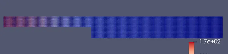
- We can see the geometry as below without grading factor
Mesh without grading Factor
Plot over line command used
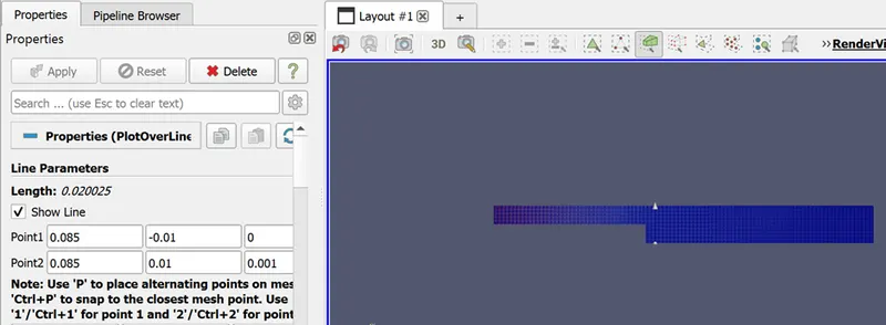
Velocity distribution along Y-axis at a distance of 0.085 from inlet
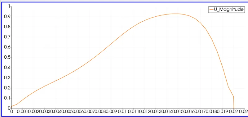
x-axis- Velocity along y direction in the geometry
y-axis- velocity in m/s
The maximum velocity reached is 0.9287 m/s and and it occurred at distance of 0.015m along Y axis.
Mesh after giving grading factor
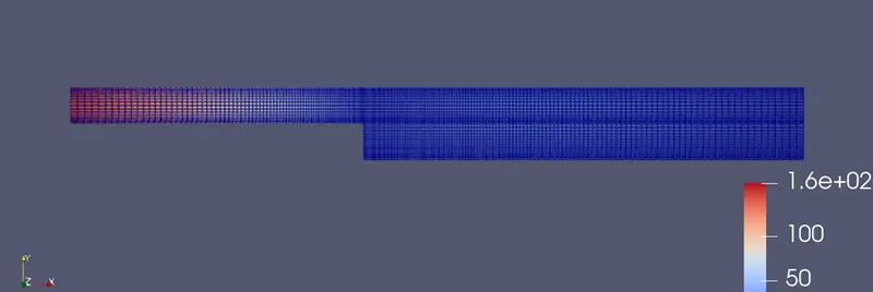
Velocity distribution along Y-axis at a distance of 0.085 from inlet with grading factor 0.2
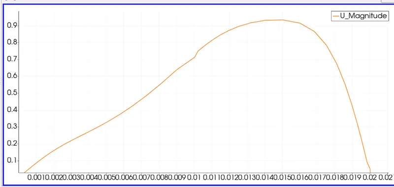
x-axis- Velocity along y direction in the geometry
y-axis- velocity in m/s
The maximum velocity reached is 0.9338 m/s and and it occurred at distance of 0.015m along Y axis.
Importance of grading factor
Grading or Growth Factor is an essential aspect of meshing because it allows for the distribution of elements of different sizes throughout the mesh. This can help to optimize the accuracy and computational efficiency of a simulation. A well-graded mesh has elements that gradually become smaller near the walls or in areas of high curvature, where higher resolution is needed to accurately capture the flow physics.
On the other hand, a poorly graded mesh with elements of similar sizes throughout can lead to poor resolution in critical areas and result in inaccurate or unreliable simulations. The growth factor is used to control the progression of element size throughout the mesh and ensure a well-graded distribution.
Conclusion
While changing the grading factor to 0.2, the mesh becomes finer in a desired location and the solution becomes accurate.
The simulation time with a grading factor in meshing can be significantly less compared to the simulation time without a grading factor. The grading factor allows for a more efficient distribution of mesh elements, where a higher density of elements is used in regions of high-gradient flow and a lower density of elements is used in regions of low-gradient flow.
This reduces the total number of elements needed to capture the flow field accurately, which leads to faster solution times and reduced computational resources. On the other hand, without a grading factor, the mesh would have an equal distribution of elements, resulting in a larger number of elements and increased simulation time.