Week 4 - CHT Analysis on Exhaust port

CHT Analysis on exhaust port

Aim:

Simulation of Conjugate Heat Transfer Analysis on Exhaust port using Ansys-Fluent.

Objective:

1. Briefly describe why and where a CHT analysis is used.

1. Maintain the y+ value according to the turbulence model and justify the results.
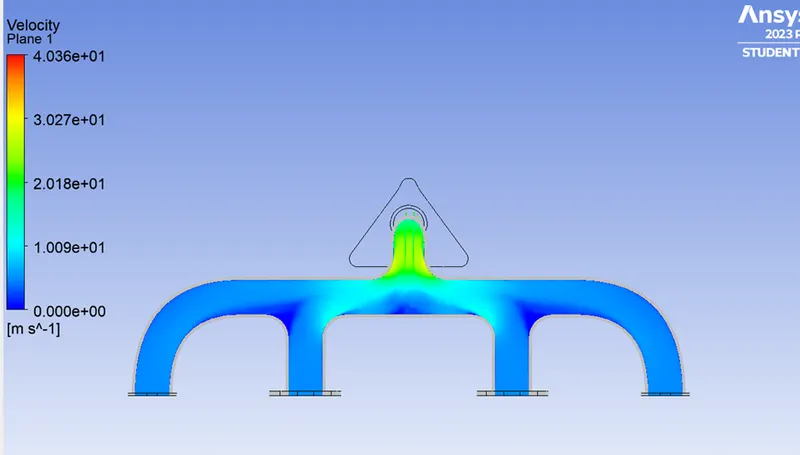
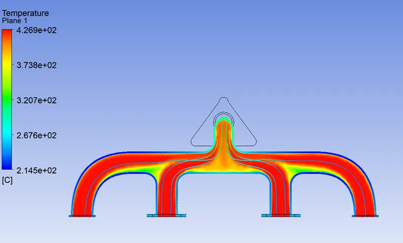
2. Calculate the wall/surface heat transfer coefficient on the internal solid surface & show the velocity & temperature contours in appropriate areas.
3. How would you verify if the HTC predictions from the simulations are right? On what factors does the accuracy of the prediction depend on?

Conjugate Heat Transfer Analysis:

Conjugate Heat Transfer (CHT) analysis is a computational technique used to study the simultaneous heat transfer between fluid flow and solid structures in a system. It involves the analysis of heat transfer within both the fluid domain and the solid domain, taking into account the interactions and exchange of thermal energy between them.

A CHT analysis is used in situations where there is a significant thermal interaction between a fluid and solid components. It is employed in a wide range of engineering applications where heat transfer plays a critical role. Here are a few examples:

1. Thermal Management of Electronics: In electronic devices such as computer chips, circuit boards, and electronic enclosures, CHT analysis helps in understanding and optimizing the heat transfer between the electronic components and the surrounding cooling mediums like air or liquid. It aids in designing effective cooling systems to prevent overheating and maintain the desired operating temperatures.
2. Aerospace and Automotive Applications: In the aerospace and automotive industries, CHT analysis is used to study the heat transfer phenomena occurring in components like engine cylinders, exhaust systems, and brake systems. It helps engineers optimize the cooling and thermal performance of these components to enhance efficiency, reduce thermal stresses, and prevent failures.
3. Power Generation Systems: CHT analysis is employed in the design and optimization of thermal power plants, including boilers, heat exchangers, and turbines. It enables engineers to understand the heat transfer characteristics within these systems, improve efficiency, and ensure safe operation.
4. Renewable Energy Systems: CHT analysis is also relevant in renewable energy systems such as solar collectors and wind turbines. It helps in understanding the heat transfer mechanisms involved, optimizing the design for maximum energy capture, and preventing overheating or structural damage.

By simulating the heat transfer interactions between the fluid and solid components, CHT analysis provides valuable insights into the thermal behavior of complex systems. It helps engineers make informed decisions, optimize designs, improve energy efficiency, and ensure various engineering applications' safe and reliable operation.

Y+ Value

The calculation of the y+ value in ANSYS Fluent involves several steps, including selecting an appropriate turbulence model and mesh resolution. Here's a general procedure for calculating the y+ value and justifying the results in ANSYS Fluent:

1. Select a Turbulence Model: ANSYS Fluent offers various turbulence models like k-ε, k-ω, Reynolds Stress Model (RSM), etc. The choice of the turbulence model affects the y+ value calculation. Different models have different requirements for the y+ value range. For instance, the k-ε model typically requires y+ values in the range of 30 to 300, while the k-ω model requires values below 1.
2. Determine the Wall Distance: Identify the wall or boundary surfaces in your simulation domain where you want to calculate the y+ value. Ensure that the mesh resolution near these walls is adequate to capture the boundary layer. In ANSYS Fluent, you can use the "Wall Distance" option to define the location of the wall.
3. Mesh Refinement: To calculate the y+ value accurately, you need to have a fine mesh near the wall. The first cell height (Δy) is crucial in determining the y+ value. It is recommended to have the first cell height less than 1% of the viscous sublayer thickness (δ). Typically, a y+ value of around 1 is desired for most turbulence models.
4. Run the Simulation: Set up the boundary conditions, turbulence model, and other required parameters in ANSYS Fluent. Then, start the simulation and let it run until convergence is achieved. Ensure that the residuals are within acceptable limits to obtain reliable results.
5. Post-Processing: Once the simulation is complete, go to the post-processing phase in ANSYS Fluent. Use the Wall Y+ tool to calculate and visualize the distribution of the y+ values on the wall surfaces. You can find this tool under the "Reports" menu.
6. Interpretation and Justification: Analyze the results and evaluate the obtained y+ values. Compare them with the recommended range for the chosen turbulence model. If the y+ values are within the desired range, it indicates that the mesh resolution near the walls is appropriate, and the turbulence model is properly capturing the flow physics. However, if the y+ values are outside the recommended range, you may need to refine or coarsen the mesh accordingly and repeat the simulation until satisfactory results are obtained.

Remember that the y+ value calculation and interpretation depend on the specific turbulence model used and the requirements of your simulation. It's important to refer to the literature or guidelines provided by ANSYS to ensure accurate calculation and justification of the y+ values for your particular case.

Geometry

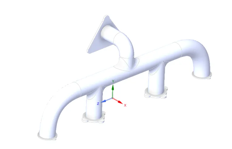
After launching geometry delete duplicate edges.

Repair --> Extra edges --> Select Extra edges --> ok

Prepare --> Volume Extract --> select edges --> ok

Rename two different volumes such as Solid Volume and Fluid Volume

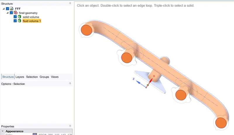
Also do the following setup in geometry.

Share Topology --> share

Workbench --> Shareprep

The above setup will ensure that we have one interface between the solid and Fluid block. If we do not make the above setting then we can’t see the interfaces where information is being shared which leads to mesh to fail.

Mesh

Named Selection

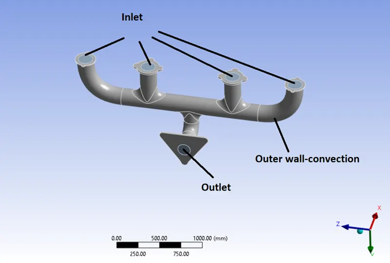
Other non-selected walls will be imported as well and by default these walls will have adiabatic Boundary condition which means these walls will not allow any heat transfer.

To generate inflation layer give named selection inflation-layer to the below selected surfaces using surface selection option.

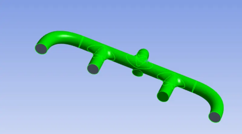
Mesh --> inflation --> All faces in chosen Named selection --> Select inflation layer

Inflation Option --> Total thickness

No. of Layer --> 5

Growth Rate --> 1.2

Maximum thickness --> 5 mm

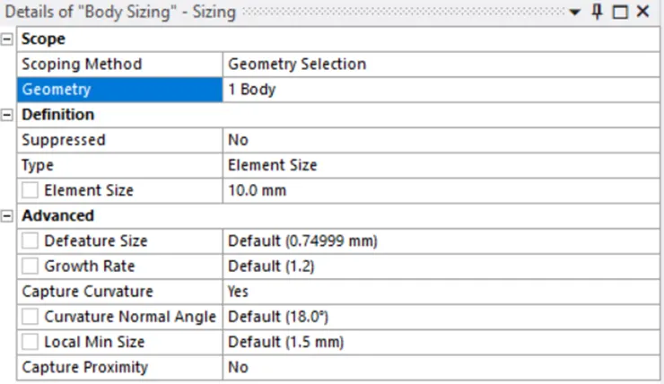
Sizing

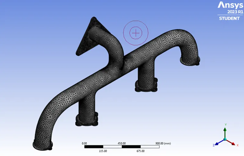
Final Mesh

Setup

Pressure-based, Absolute and steady state

Energy equation enables as we are dealing with temperature

Viscous --> k-ω model

Boundaries --> inlet --> 5 m/s, 700K

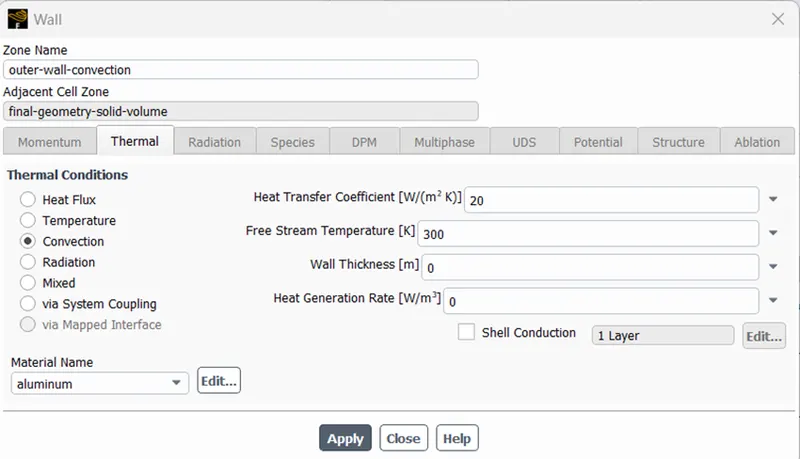
Boundaries --> outer-wall-convection --> Thermal

Thermal condition – Convection, Heat Transfer Coefficient – 20 W/(m² K)

k-ω turbulence model:

The k-ω turbulence model is commonly used in computational fluid dynamics (CFD) simulations in various engineering applications. Here are some situations where the k-ω model is typically preferred:

1. Wall-Bounded Flows: The k-ω model is well-suited for simulating wall-bounded flows, such as turbulent boundary layers and flows over solid surfaces. It accurately predicts the near-wall behavior and captures the effects of wall shear stress on the turbulence characteristics. The model is particularly effective in cases where the flow exhibits adverse pressure gradients, separation, or reattachment.
2. Strong Curvature or Rotational Flows: The k-ω model performs well in flows with strong curvature or rotational effects. Examples include flows around curved surfaces, swirling flows, and rotating machinery. The model's capability to account for rotational effects helps in capturing the complex flow patterns and secondary flows that arise in such situations.
3. Low-Reynolds Number Flows: The k-ω model is suitable for low Reynolds number flows, where the viscous effects dominate over the turbulent effects. It accurately predicts the near-wall behavior and avoids excessive dissipation, making it suitable for laminar-to-turbulent transition simulations or cases with low turbulence intensity.
4. Flow Separation and Recirculation: The k-ω model handles flow separation and recirculation regions reasonably well. It captures the formation and behavior of eddies and vortices in these areas, making it beneficial for simulating flows with complex flow separation patterns.

Results

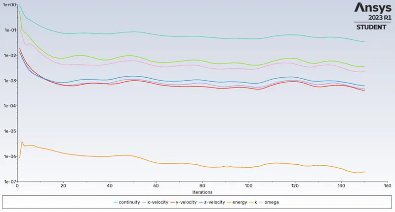
Scaled Residuals

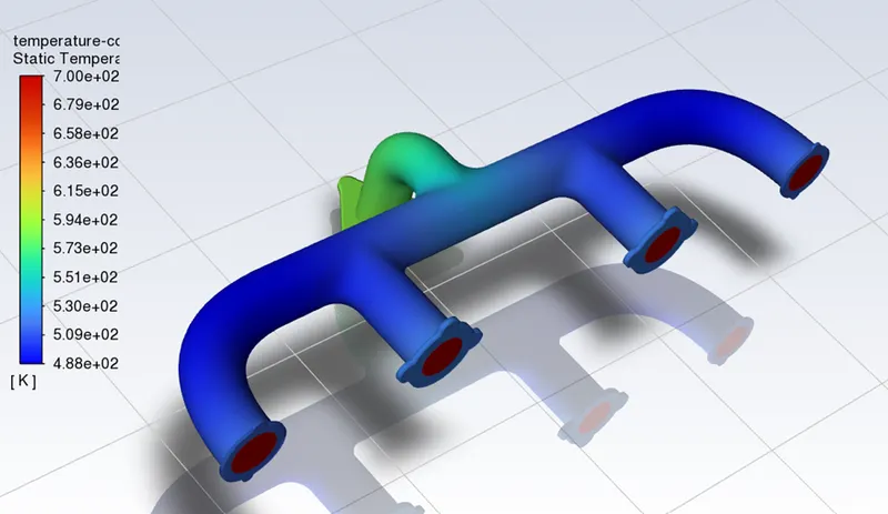
Temperature contour

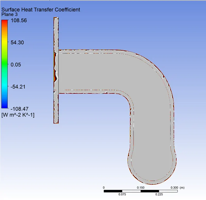
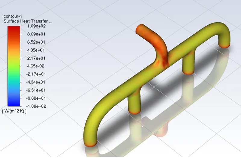
Surface Heat transfer coefficient

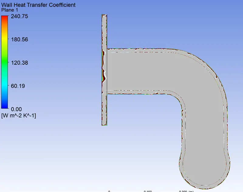
Wall Heat transfer Coefficient

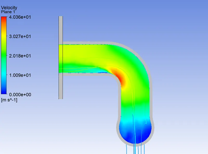
Velocity contour

Temperature contour

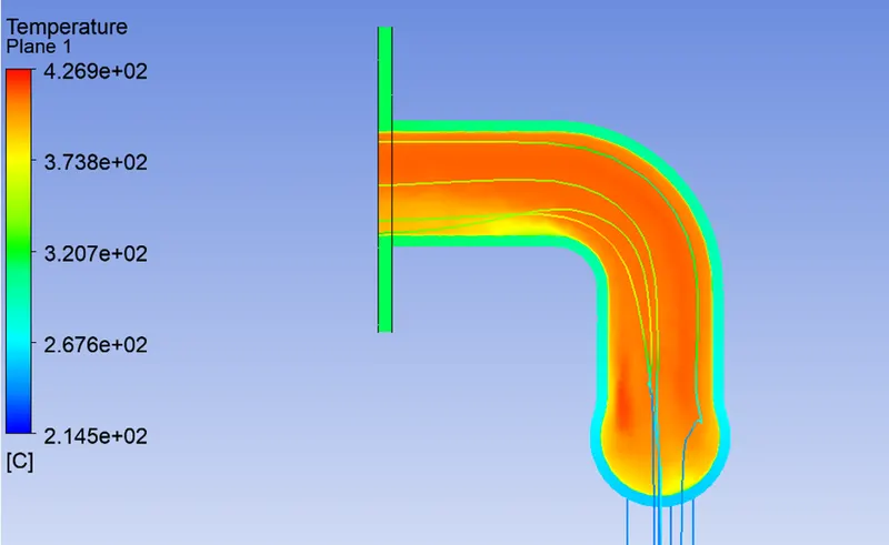
Surface Heat transfer Coefficient

Surface Heat Transfer Coefficient = -28.268115 W/(m^2 K)

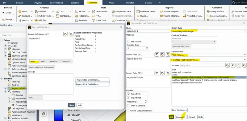
Wall Heat transfer Coefficient

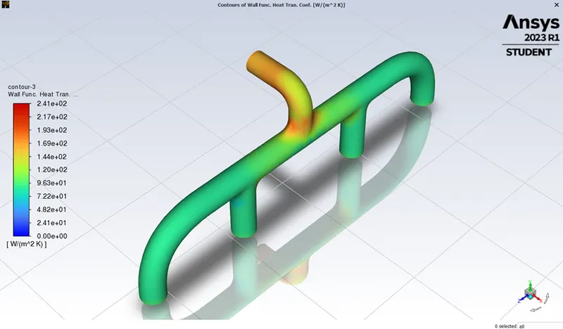
Wall Heat transfer coefficient = 101.537 W/(m^2 K)

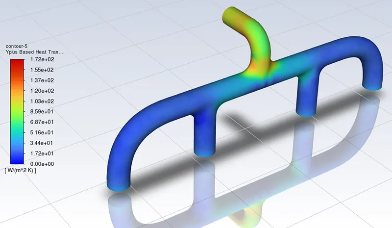
Y+ based on Heat transfer coefficient

On what factors does the accuracy of the prediction depend on?

The accuracy of predictions in simulations depends on several factors. Here are some key factors that influence the accuracy of predictions:

1. Model Validity: The accuracy of predictions heavily relies on the validity of the mathematical model used in the simulation. The model should appropriately represent the physical phenomena and governing equations relevant to the problem being studied. Assumptions and simplifications made in the model should be justified and appropriate for the specific application.
2. Input Data: The accuracy of input data, such as boundary conditions, initial conditions, material properties, and geometric details, directly impacts the accuracy of predictions. It is important to use reliable and accurate data obtained from experiments, measurements, or validated sources. Any uncertainties or errors in input data propagate through the simulation, affecting the overall accuracy.
3. Mesh Resolution: The mesh resolution plays a critical role in capturing the flow and temperature gradients accurately. A fine mesh is necessary near boundaries, regions of interest, or areas with strong variations in flow or temperature. Inadequate mesh resolution may lead to inaccurate predictions, especially in areas where significant changes occur, such as boundary layers or flow separation regions.
4. Turbulence Modeling: Turbulence models are used to simulate turbulent flows, and their accuracy affects the predictions. The choice of a turbulence model should be based on the specific flow conditions and geometries involved. It is important to select an appropriate turbulence model and validate its performance against experimental or reference data to ensure accurate predictions.
5. Numerical Methods and Convergence: The numerical methods employed in the simulation, such as discretization schemes and solution algorithms, can affect the accuracy. The use of appropriate numerical methods that ensure convergence, stability, and conservation of the governing equations is crucial for obtaining accurate predictions.
6. Experimental Validation: Comparing simulation results with reliable experimental data or analytical solutions is an essential step in assessing accuracy. Experimental validation helps to verify the simulation setup, identify discrepancies, and gain confidence in the predictions.
7. Sensitivity Analysis: Conducting sensitivity analyses to evaluate the impact of various parameters on the predictions provides insights into the uncertainties and their effects. Assessing the sensitivity of predictions to changes in boundary conditions, material properties, or modeling choices helps to understand the robustness and accuracy of the simulations.
8. Engineering Expertise: The accuracy of predictions also depends on the expertise and knowledge of the engineer conducting the simulation. Understanding the physics of the problem, selecting appropriate modeling approaches, and making informed judgments during the simulation process contribute to accurate predictions.

It is important to note that achieving absolute accuracy in simulations is often challenging, and there are inherent limitations and uncertainties associated with any modeling and simulation process. However, by considering and optimizing these factors, the accuracy of predictions can be significantly improved.

Conclusion:

Simulation of CHT Analysis on exhaust port is done. The Various application of CHT analysis is explained briefly and the factors affecting the accuracy of predictions in simulation were explained.