Week 1- Mixing Tee
Mixing Tee
Aim:
Set up Steady-state simulations to compare the mixing effectiveness when hot and cold air enters into the Tee joint.
Problem Statement:
The hot inlet temperature is 360C & the Cold inlet is at 190C.
Use the k-epsilon and k-omega SST model for the first case and based on your judgment use the more suitable model for further cases. Giving the reason for choosing a suitable model is compulsory.
- Case 1
- Short mixing tee with a hot inlet velocity of 3m/s.
- Momentum ratio of 2, 4.
- Case 2
- Long mixing tee with a hot inlet velocity of 3m/s.
- Momentum ratio of 2, 4.
Momentum ratio = velocity at cold inlet / velocity at hot inlet
Mixing Tee – Application:
A mixing tee is a pipe fitting that is used to combine two or more fluid streams into a single stream. This type of tee is commonly used in process piping systems in industries such as chemical, pharmaceutical, and food and beverage.
The application of a mixing tee is to ensure that the fluids being mixed are combined in a uniform manner, with each fluid contributing to the mixture in a consistent and proportional way. The mixing tee achieves this by redirecting the flow of each fluid and combining them in a specific ratio to achieve the desired mixture.
One common application of a mixing tee is in the blending of two different chemicals in a chemical process. The mixing tee can be used to control the ratio of the two chemicals being blended and ensure that they are thoroughly mixed before being further processed.
Another application of a mixing tee is in the production of food and beverage products. For example, a mixing tee can be used to combine different ingredients in a recipe, such as milk and sugar, to create a homogenous mixture that can be further processed into a finished product.
Overall, the mixing tee is a versatile pipe fitting that is used in a wide range of applications to ensure that fluids are blended in a consistent and uniform manner.
Ansys WorkBench for fluid flow problems:
In this problem we use ANSYS Workbench, which is a software tool used for simulating and analyzing fluid flow problems. It is a comprehensive platform that allows engineers to set up, solve, and analyze complex fluid flow problems with ease. Here are the key features of ANSYS Workbench for fluid flow problems:
Geometry creation: ANSYS Workbench provides a suite of geometry tools that enable engineers to create and modify complex geometries. It supports 2D and 3D geometries and offers various methods for geometry creation, such as parametric design, CAD import, and scripting.
Meshing: ANSYS Workbench offers advanced meshing capabilities, allowing engineers to generate high-quality meshes for fluid flow problems. It supports a wide range of meshing techniques, including structured, unstructured, and hybrid meshes. The software also provides tools for mesh refinement and optimization.
Physics setup: ANSYS Workbench supports a wide range of physics models for fluid flow problems, including laminar, turbulent, and multiphase flows. The software also allows users to specify boundary conditions, such as velocity, pressure, and temperature.
Solver: ANSYS Workbench uses the ANSYS Fluent solver for simulating fluid flow problems. The Fluent solver is a highly accurate and robust solver that can handle a wide range of fluid flow problems.
Post-processing: ANSYS Workbench provides a suite of post-processing tools that enable engineers to visualize and analyze simulation results. The software supports various types of plots, including contour plots, vector plots, and streamline plots. It also provides tools for data analysis, such as statistics and time averaging.
Overall, ANSYS Workbench is a powerful software tool for simulating and analyzing fluid flow problems. Its user-friendly interface and advanced capabilities make it a popular choice among engineers and researchers in the field of fluid dynamics.
Case 1a:
Short Mixing Tee with MR=2, k-epsilon model
Hot inlet Temperature – 360 C
Cold inlet Temperature – 190 C
Hot inlet Velocity – 3 m/s
Cold inlet Velocity – 6 m/s
Let us start with Ansys Workbech and double click on Fluid Flow (fluent) on the left side Tool box and Rename it as Mixing Tee_short_MR=2.
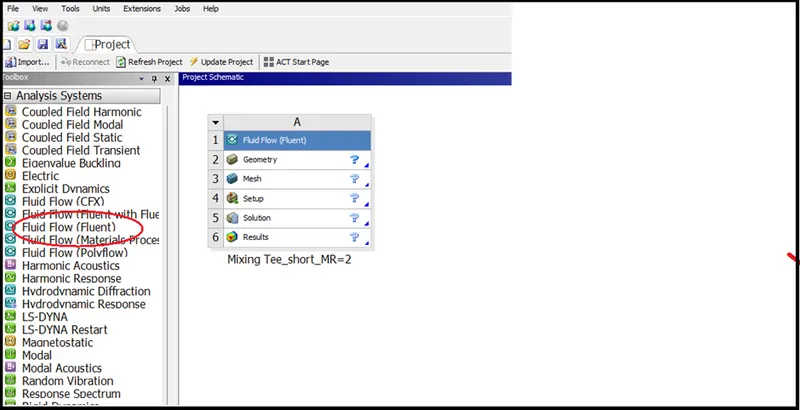
Double click on Geometry to load the Short Tee cad model using Ansys Discovery and SpaceClaim.
ANSYS Discovery and SpaceClaim are software tools that can be used to load CAD models into ANSYS Workbench for further simulation and analysis
Once the model is loaded we need to extract the required parts alone to run the simulation which can be done by Prepare à Volume Extract à Edges as shown below. And select the edges that are needed for our simulation.
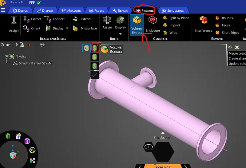
After Extraction
Now close the Ansys Discovery and go back to Workbench, double click on Mesh.
Meshing [CFD PrepPost] will be opened, right click on Mesh located in the left side panel and give generate Mesh, and keep the default element size as highlighted below.
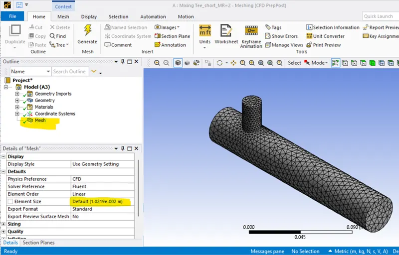
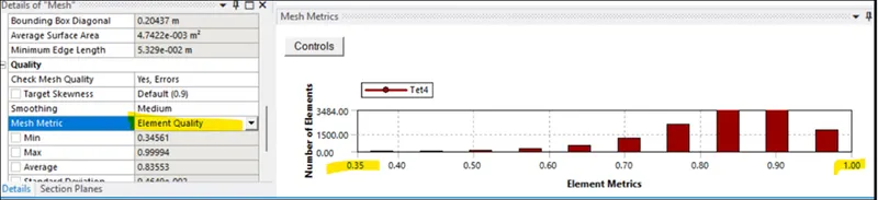
To check the Quality of the Mesh click on Quality --> Mesh Metric --> Element Quality.
Element quality refers to how well the mesh elements represent the physical shape of the geometry being meshed. Element quality is a measure of how closely the elements conform to the ideal shape for the type of element being used. An element with good quality will have a shape that closely resembles the ideal shape for that element type, which can improve the accuracy and stability of the CFD simulation. Conversely, an element with poor quality will have a distorted shape that can lead to numerical errors and inaccurate results.
In General element quality should not be less than 5%. In the screen shot below, the left side 0.35 represents 35% and the right corner represents 100%.
Now click on face selection and right-click on the face that we need to define the boundary name as shown below.
Give inlet-y for the cold inlet and inlet-x for the hot inlet and for the exit give ‘outlet’ to identify the faces for our simulation.
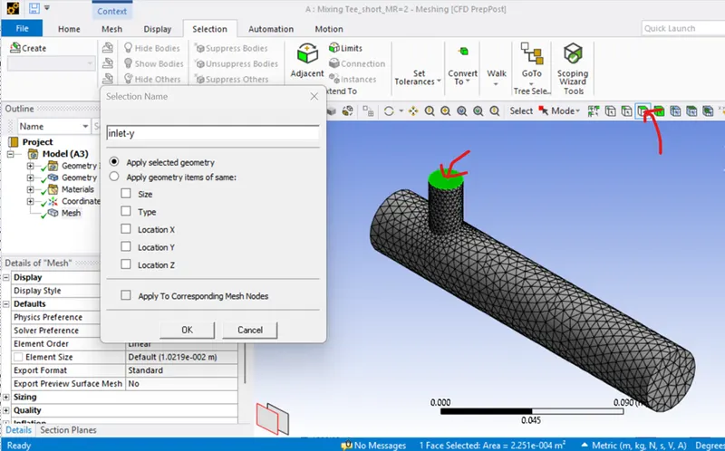
Then close meshing and return to workbench. Before opening the setup right click on Mesh and give update.
Once we double-click on setup Fluent Launcher will be opened. Select Double Precision and start.
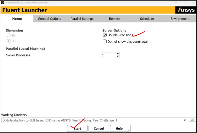
When launching ANSYS Fluent, the user is presented with a Windows-based graphical user interface (GUI) that allows for easy input of simulation parameters and post-processing of results.
The main ANSYS Fluent GUI consists of several windows:
- Project Schematic window: This is the main window where the user can create and manage simulation projects. Here, the user can define the simulation domain, boundary conditions, solver settings, and post-processing options.
- Outline View window: This window allows the user to give input values for the simulation
- Task Page Window: It consists of general settings to choose for the simulation.
- Console window: This window displays the status of the ANSYS Fluent solver as it runs the simulation. Any run time error will be displayed in the console window.
- Toolbar: The toolbar provides quick access to commonly used functions, such as saving the project, running the simulation, and exporting results.
- Menus: The menus provide access to all of the ANSYS Fluent functions, including meshing tools, solver settings, and post-processing options.
The first step is to check Mesh. Click on Check --> Perform Mesh Check. We can see checking Mesh and Done in console.
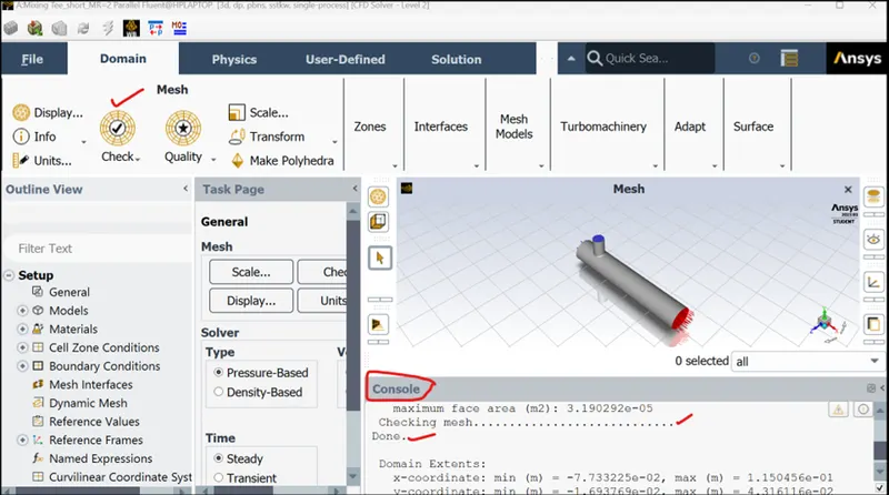
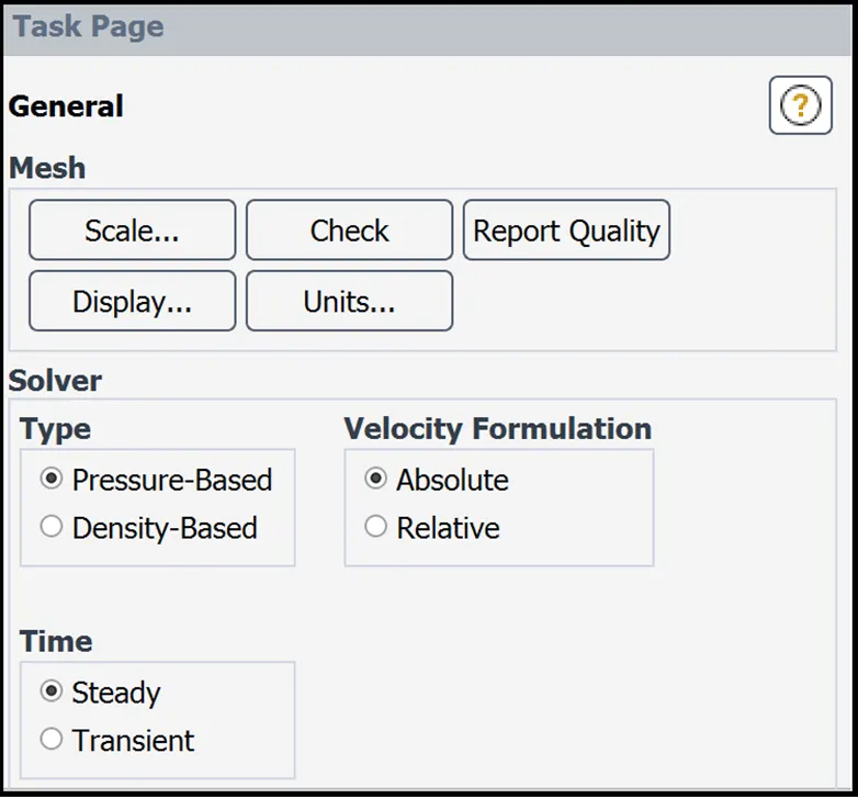
In the task Page we need to choose Pressure-Based, Absolute and Steady as shown below.
Pressure-based solver is most commonly used solver in ANSYS Fluent and is well-suited for incompressible and low-speed compressible flows.
In the absolute Velocity formulation, the fluid velocity is defined relative to an absolute reference frame, rather than to a moving or rotating reference frame.
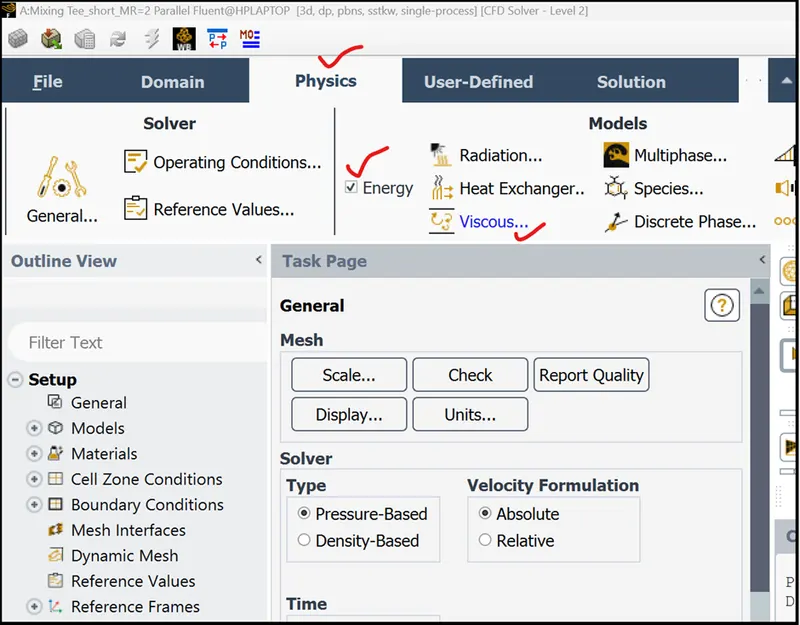
Then move to Physics, Click on Energy Equation.
The energy equation is an important equation in fluid dynamics that relates the temperature, pressure, and velocity fields of a fluid. In ANSYS Fluent, the energy equation is solved to determine the temperature field of a fluid, and it is typically included in simulations when thermal effects are important to the problem being modelled.
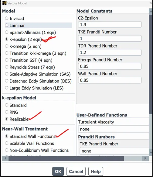
Now select Viscous model --> K-epsilon --> Realizable --> Standard wall function
K-epsilon model is one of the most commonly used turbulence models in industry and academia due to its computational efficiency and accuracy in a wide range of flow regimes.
The k-epsilon model is a two-equation model, where two additional transport equations are solved for the turbulent kinetic energy (k) and the rate of dissipation of turbulent kinetic energy (epsilon). These equations are solved alongside the governing equations of mass, momentum, and energy conservation to obtain a complete solution for the fluid flow problem.
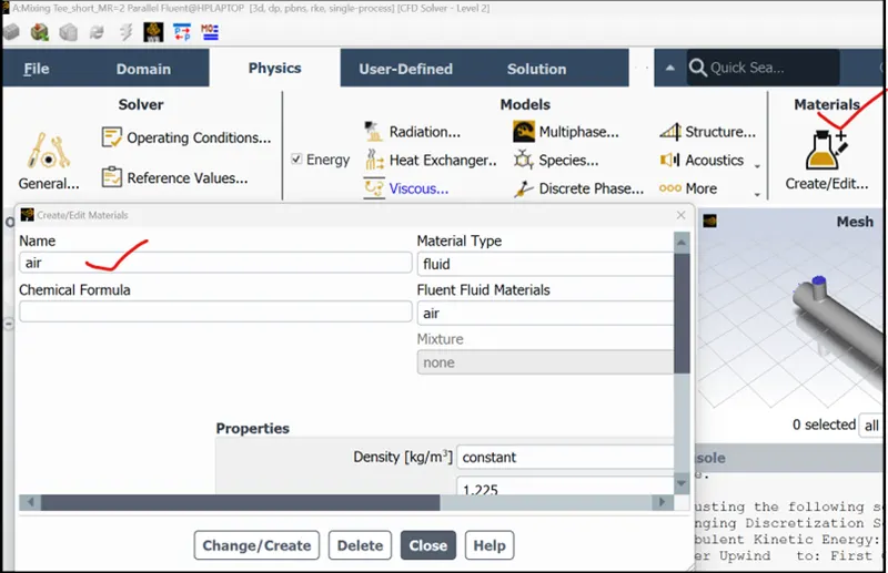
Then choose the Material Air from the toolbar located above.
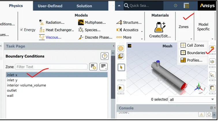
Now click on Zones --> Boundaries -->inlet-x -->Edit (located at the bottom)
Inlet-x – Velocity = 3 m/s, and Temperature = 360 C
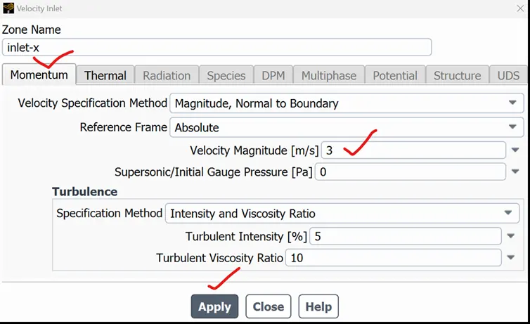
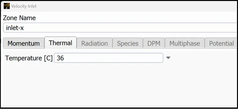
Inlet-y – Velocity = 6 m/s, and Temperature = 190 C
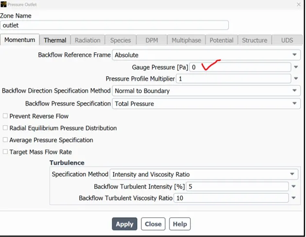
For Outlet type should be Pressure out and Gauge pressure should be 0.
Then click on Definitions --> New --> Surface Report --> Area weighted Average.
Then choose the options as shown in the below screenshots to get the temperature and Velocity plot.
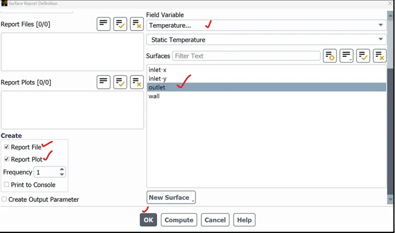
Click on Definitions --> New --> Surface Report --> Standard deviation, then select Temperature in the Field Variable and Outlet in Surfaces.
Then click on Solution --> Initialization --> Initialize. We can check the Initialization done in Console window as shown below.
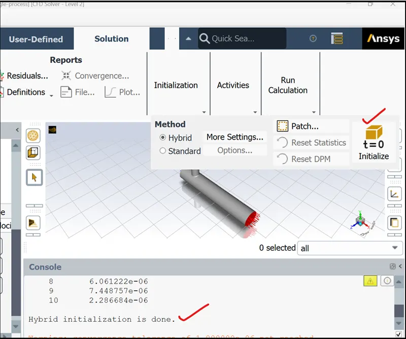
Initialization is an important step in ANSYS Fluent that involves setting the initial conditions for the fluid flow simulation. The purpose of initialization is to provide the solver with a starting point for the solution, so that the simulation can converge to a stable solution more quickly and accurately.
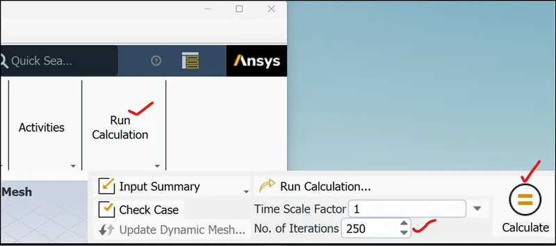
Then run simulation with 250 iterations.
Results
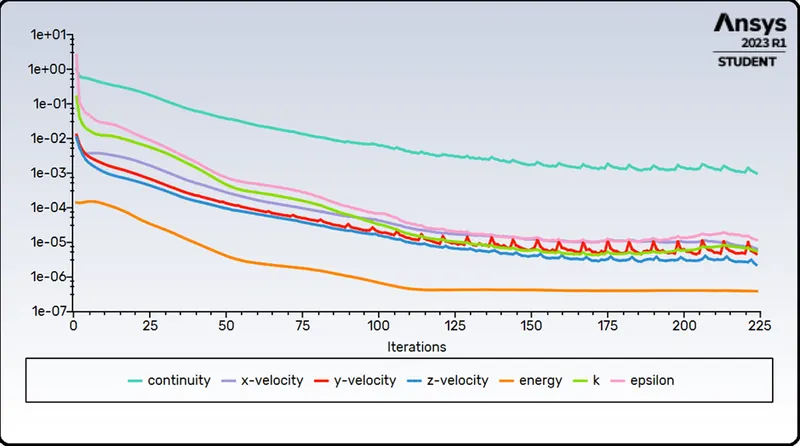
Scaled Residuals
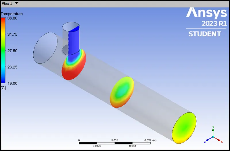
Temperature Plot
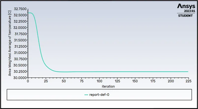
Solution converged at 223th iteration and the Temperature at the Outlet reached 30.240 C
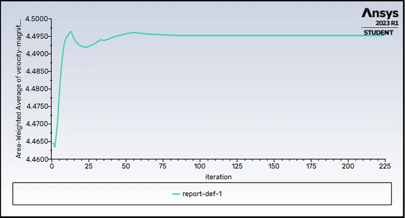
Velocity Plot
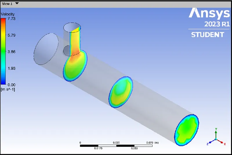
Solution for Velocity converged approximately at 225th iteration and Velocity reached 4.50 m/s
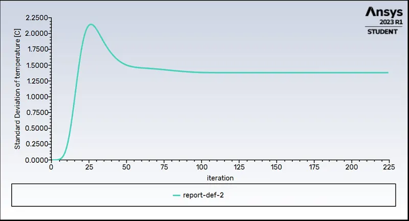
Standard deviation for Temperature
Standard deviation is 1.38050 C reached at 222th iteration.
Close Ansys fluent and return to workbench. Click on Results
You will be seeing CFD Post with Wireframe in the beginning, click on wall on the left side Panel to see the model.
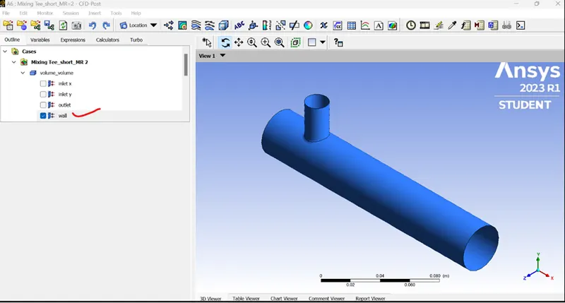
Double Click on Wall -->Color --> select White, so that we can see the temperature and Velocity contour clearly.
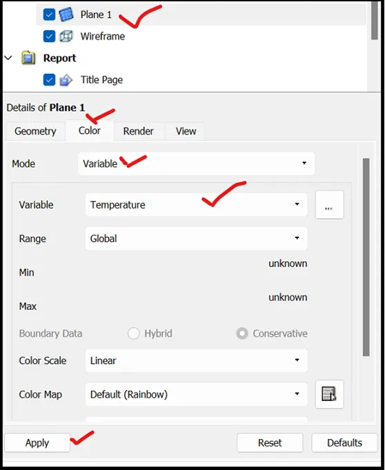
Insert --> Location --> Plane --> Plane 1 (Name) --> OK
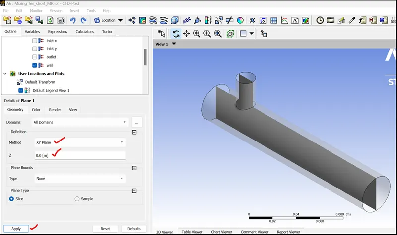
Color --> Mode --> Variable --> Variable --> Temperature --> apply
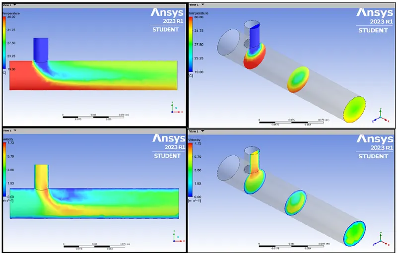
Temperature Contour
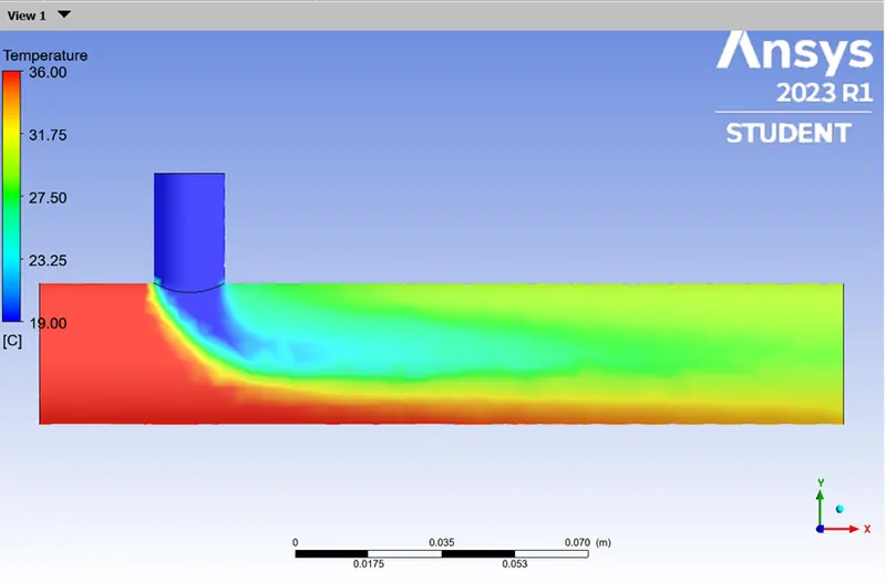
Temperature Contour across the pipe
Velocity Contour
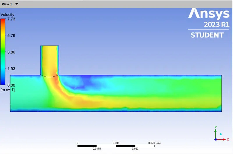
Velocity contour Across the Pipe
Row 1: Temperature contour
Row 2: Velocity Contour
Case 1b:
Short Mixing Tee with MR=2, k-omega model
Hot inlet Temperature – 360 C
Cold inlet Temperature – 190 C
Hot inlet Velocity – 3 m/s
Cold inlet Velocity – 6 m/s
k-omega Model:
The k-omega SST model is a two-equation model that solves transport equations for turbulent kinetic energy (k) and the specific dissipation rate of turbulent kinetic energy (omega). The model also includes additional transport equations for the turbulent viscosity and a new variable called the shear strain rate, which represents the rate of strain in the direction of the velocity gradient.
The k-omega SST model combines the benefits of the k-epsilon and k-omega models. It uses the k-epsilon model to calculate the turbulence viscosity in the near-wall region, where viscous effects are dominant, and the k-omega model to model the free-stream turbulence in the outer flow region. This hybrid approach makes the k-omega SST model well-suited for simulating a wide range of flow conditions, including boundary layers, wakes, jets, and separated flows.
For case 1b
Average temperature reached at outlet = 30.280 C , reached at 600th iteration
Velocity at outlet = 4.50 m/s, reached at 600th iteration
Standard deviation = 1.3503, reached at 597th iteration.
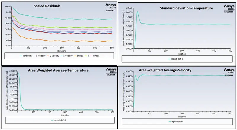
Temperature and Velocity Contour plots for Short Tee, MR=2, k-omega model
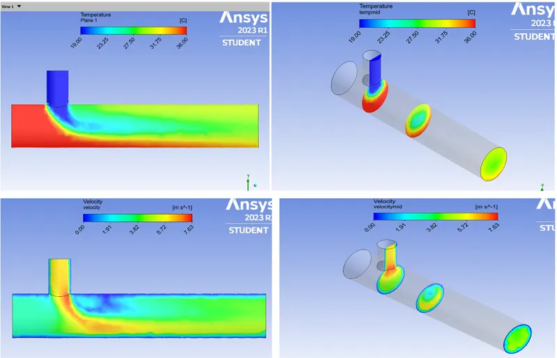
Difference between k-epsilon and k-omega model
The k-epsilon and k-omega turbulence models are both two-equation models widely used in computational fluid dynamics (CFD) to simulate turbulent flows. The main difference between them is in the way they model the turbulent viscosity and the dissipation of turbulence kinetic energy.
The k-epsilon model solves transport equations for turbulent kinetic energy (k) and the rate of dissipation of turbulence kinetic energy (epsilon). The model assumes that the turbulent viscosity is proportional to k and epsilon, and that the dissipation of turbulent kinetic energy is primarily caused by the viscous effects.
The k-omega model, on the other hand, solves transport equations for turbulence kinetic energy (k) and the specific dissipation rate of turbulence kinetic energy (omega). The model assumes that the turbulent viscosity is proportional to k and omega, and that the dissipation of turbulent kinetic energy is primarily caused by the turbulence itself.
Both models have their own advantages and disadvantages. The k-epsilon model is easier to implement and computationally less expensive than the k-omega model. It is also more suitable for simulating boundary layer flows and flows with moderate Reynolds numbers. However, the k-epsilon model has some limitations, such as its inability to accurately predict flows with high levels of turbulence or flows with strong streamline curvature.
The k-omega model is more accurate than the k-epsilon model in predicting turbulent flows with high levels of turbulence or flows with strong streamline curvature. It is also more suitable for simulating flows in complex geometries or flows with adverse pressure gradients. However, the k-omega model requires more computational resources than the k-epsilon model due to its additional transport equation.
For steady-state simulations, either k-epsilon or k-omega model can be used depending on the specific flow conditions and the level of accuracy required. In general, the k-epsilon model is preferred for simpler and moderate flow conditions, while the k-omega model is preferred for complex and highly turbulent flows. So for further cases we will be using k-epsilon model for our problem.
Case 1c:
Short Mixing Tee with MR=4, k-epsilon model
Hot inlet Temperature – 360 C
Cold inlet Temperature – 190 C
Hot inlet Velocity – 3 m/s
Cold inlet Velocity – 12 m/s
Average temperature reached at outlet = 27.53060 C , reached at 171th iteration
Velocity at outlet = 6.0151 m/s, reached at 168th iteration
Standard deviation = 0.9749, reached at 165th iteration
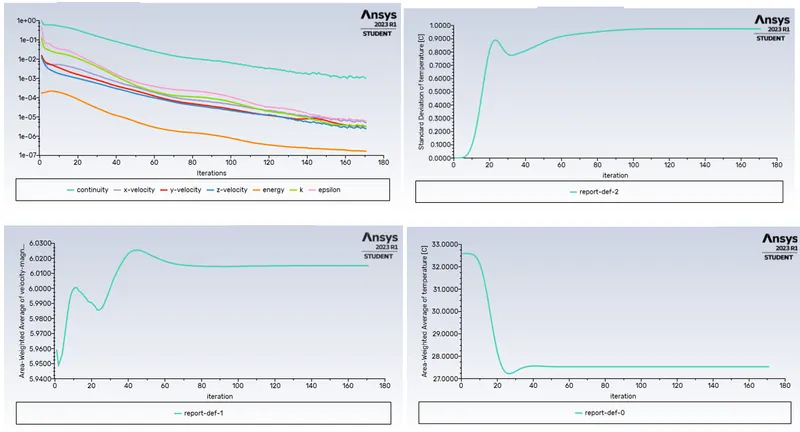
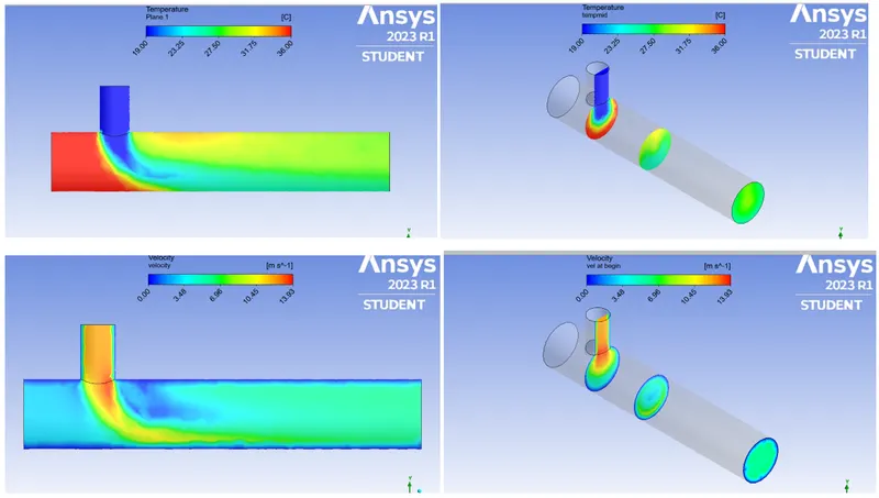
Temperature and Velocity Contour plots for Short Tee, MR=4, k-epsilon model
Case 2a:
Long Mixing Tee with MR=2, k-epsilon model
Hot inlet Temperature – 360 C
Cold inlet Temperature – 190 C
Hot inlet Velocity – 3 m/s
Cold inlet Velocity – 6 m/s
Average temperature reached at outlet = 30.310 C , reached at 171th iteration
Velocity at outlet = 4.49 m/s, reached at 171th iteration
Standard deviation = 0.7636, reached at 171th iteration
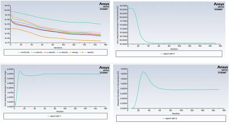
Temperature and Velocity Contour plots for Long Tee, MR=2, k-epsilon model
Case 2b:
Long Mixing Tee with MR=4, k-epsilon model
Hot inlet Temperature – 360 C
Cold inlet Temperature – 190 C
Hot inlet Velocity – 3 m/s
Cold inlet Velocity – 12 m/s
Average temperature reached at outlet = 27.480 C , reached at 155th iteration
Velocity at outlet = 6 m/s, reached at 156th iteration
Standard deviation = 0.7673, reached at 156th iteration
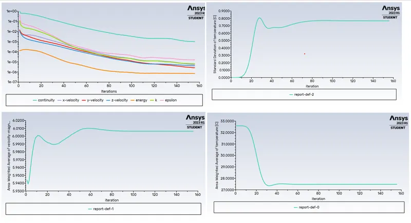
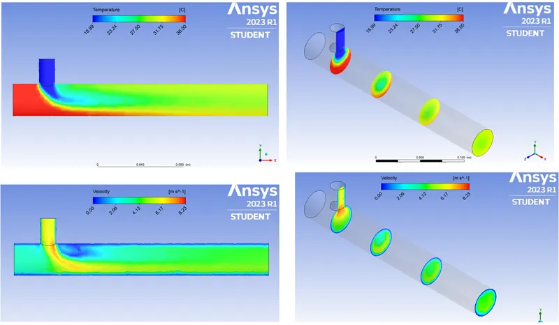
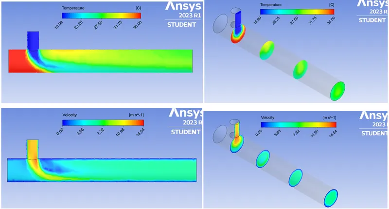
Temperature and Velocity Contour plots for Long Tee, MR=4, k-epsilon model
Result
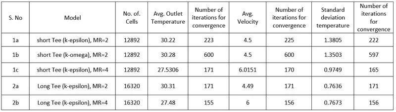
Comparing all the models together short Tee with MR=4 is efficient. Short Tee with MR=4, and Long Tee with MR=4 both gives almost same result.
So Increasing the length of Mixing Tee doesn’t have much effect on Temperature.
Also comparing the material cost, we can have short Tee with higher velocity at inlet-y to get the maximum efficiency.
Grid Independence Test

From the above table the average Velocity and temperature are approximately equal while increasing the number of cells for case 1.
Hence the solution of Mixing Tee_short, is Grid independent.