Week 6 - CHT Analysis on a Graphics card

AIM: Perform a steady-state conjugate heat transfer analysis on a model of a graphics card.

Objective:

1. Run the simulation by varying the velocity from 1m/sec to 5m/sec for at least 3 velocities and discuss the results.
2. Find out the maximum temperature and heat transfer coefficient attained by the processor.
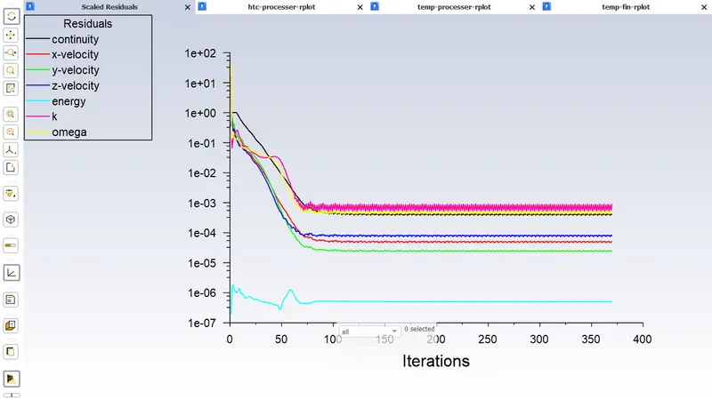
3. Prove that the simulation has achieved convergence with appropriate images and plots.
4. Identify potential hotspots on the model.

Theory:

Heat:

Heat is a form of energy that exist due to the temperature difference. Heat transfer can be defined as the transmission of energy from one region to another region as a result of temperature difference.

There are three basic modes of heat transfer.

1. Conduction: This is the mode of heat transfer in which energy exchange takes place due to temperature difference by kinetic motion, direct impact of molecules example metals
2. Convection: This is the mode of heat transfer in which energy exchange takes place due to the temperature difference by the macroscopic motion of fluid particles.

• Radiation: This is the mode of heat transfer in which the energy exchange takes place without the aid of any intervening medium.

Fourier Law of heat transfer:

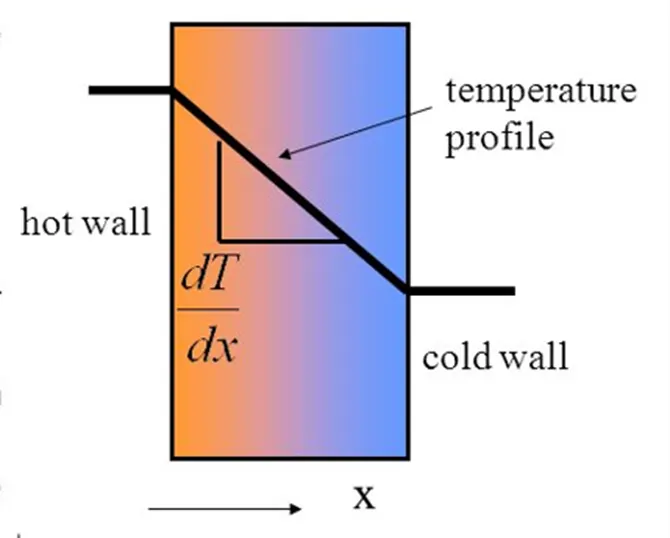
The law of heat conduction based on experimental observation is known as the Fourier’s Law which state that “ The rate of heat flow by conduction in a given direction is proportional to the area normal the direction of the heat flow and also temperature gradient in that direction”.

It is given by the below formula

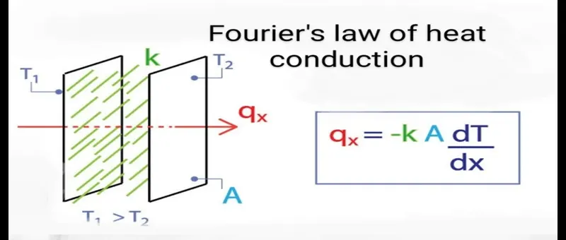
Where qx is the rate of heat flow in Watts or J/s

A is the areas normal to the direction of heat transfer in m2

dT/dx is the Temperature gradient in °K/m

-ve sign indicated that heat flows from higher temperature to lower temperature.

k, is called thermal conductivity of the material, it is the property of the material which varies with temperature.

Thermal conductivity (k):

Thermal conductivity of a metal can be define as the rate of heat transfer through a unit thickness of the material per unit area per unit temperature difference.

The unit of Thermal conductivity is W/m-°K

A higher the value of thermal conductivity indicates that the material is good heat conductor and low value indicates poor heat conductor or insulator.

Newtons Cooling Law:

It states that convective heat transfer is proportional to the difference in temperature between an object and its surrounding area.

It is given by the below formula

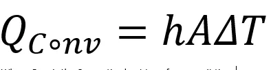
Where QConv is the Convective heat transfer per unit time

h is the heat transfer coefficient W/m2 °K

A is the Normal surface area in m2.

^T is the temperature difference in °K

Convective is a mode of energy transfer that involves the combine effect of conduction and fluid motion between the solid surface and an adjacent moving liquid or gas.

Faster the fluid flow higher the convective heat transfer.

Thermal diffusivity:

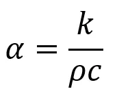
Thermal diffusivity is the measure of the ratio of heat conducted to the heat stored and consequently can be used qualitatively to predict how fast the temperature of the body changes. A material.

It is given by the below equation:

Where α is the thermal diffusivity in m2/s

k is Thermal conductivity in W/m-°K

𝜌 is the density in kg/m3

C is the Specific heat capacity in kJ/kg °K

The larger values of α for higher value of k and lower value of 𝜌c leads to the faster heat dissipation in the material.

Higher the value of k will result in the faster energy transfer though the material

Lower the value of c means lesser amount of heat moving through the material will be used for raising the temperature and more of it will be available for transferring.

Specific heat capacity (c) :

Specific heat capacity is defined as the amount of energy require to rise the temperature by 1 °C per unit kg of the substance.

Its SI unit is KJ/kg °K

There are 2 types of convection heat transfer.

• Forced convection
• Free or Natural convection

1) Forced convection

When a fluid is forced to flow over the surface by an internal source such as fans, by stirring, and pumps, creating an artificially induced convection current

2) Free or Natural convection

The mechanism of heat transfer in natural convection involves the motion of fluid particles past a solid boundary which is a result of the density differences resulting from the energy exchange. As a result, the heat transfer coefficients will vary with the geometry

“h” heat transfer coefficient is not a property it’s a experimentally determined parameter like temperature, surface geometry and velocity of the fluid.

Fins:

The rate of heat transfer from a surface at a temperature 𝑇𝑠 to the surround in medium at 𝑇∞ is given by Newton’s law of cooling as

𝑄𝑐𝑜𝑛𝑣 = ℎ𝐴𝑠(𝑇𝑠 − 𝑇∞)

where 𝑨𝒔 is the heat transfer surface area and h is the convection heat transfer coefficient. When the temperatures 𝑻𝒔 and 𝑻∞ are fixed by design considerations, as is often the case, there are two ways to increase the rate of heat transfer: to increase the convection heat transfer coefficient 𝒉 or to increase the surface area 𝑨𝒔. Increasing h may require the installation of a pump or fan, or replacing the existing one with a larger one, but this approach may or may not be practical. Besides, it may not be adequate. The alternative is to increase the surface area by attaching to the surface extended surfaces called fins made of highly conductive materials such as aluminum. Finned surfaces are commonly used in practice to enhance heat transfer, and they often increase the rate of heat transfer from a surface several fold.

Fins are often seen in electrical appliances and electronics such as on computer processors and power supplies and industrial applications such as heat exchangers and substation transformers.

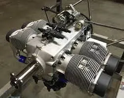
Examples: Light weight 4 cylinder Aircraft engine as shown below picture.

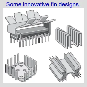
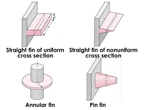
Please refer the below photos for the types of fins.

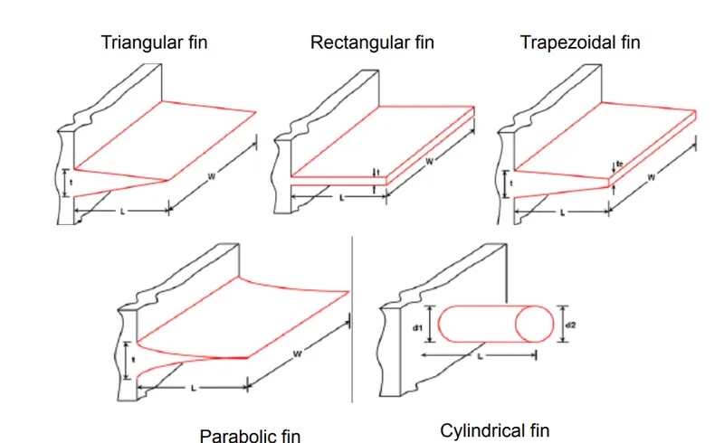
Following are the performance characteristics of the fin:
1) Temperature distribution
2) Rate of heat transfer
3) Fin efficiency

Following are the assumptions made for differential heat equation for a fin
1. Steady state
2. One dimensional
3. Uniform convective heat transfer coefficient
4. Constant thermal conductivity

Differential heat equation for a fin is given by

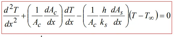
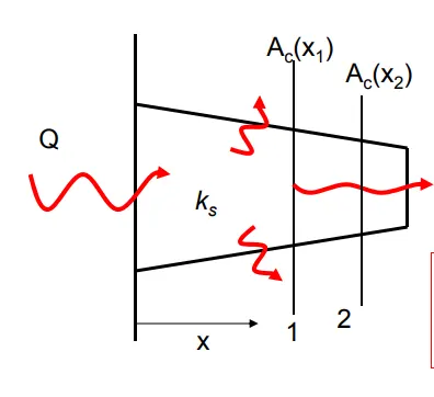
Whare Ac(x) is cross sectional area Heat conducted through this area inside the fin

Ks is the thermal conductivity of solid.

T and Tinfinite are te temperature of the solid and temperature of infinite length of fin.

On simplyfining the obove differential heat equation we get

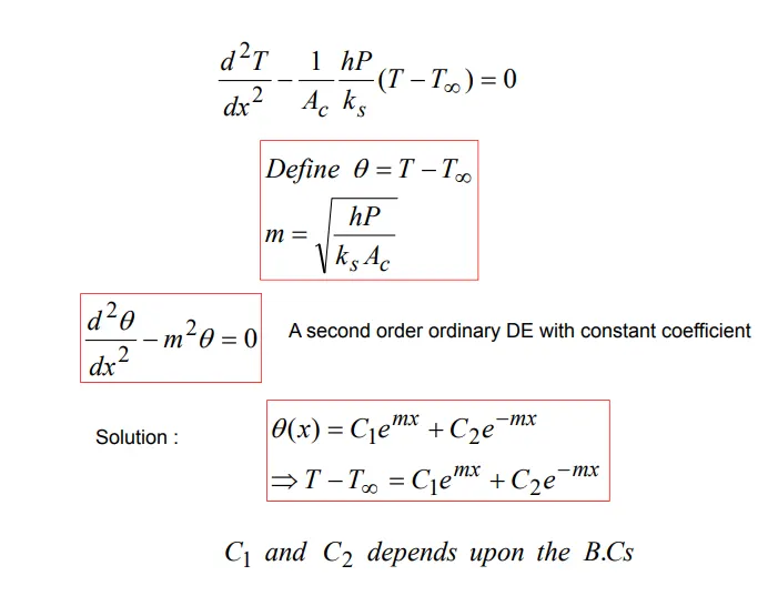
Please refer the below photo for the General Boundary Conditions applied.

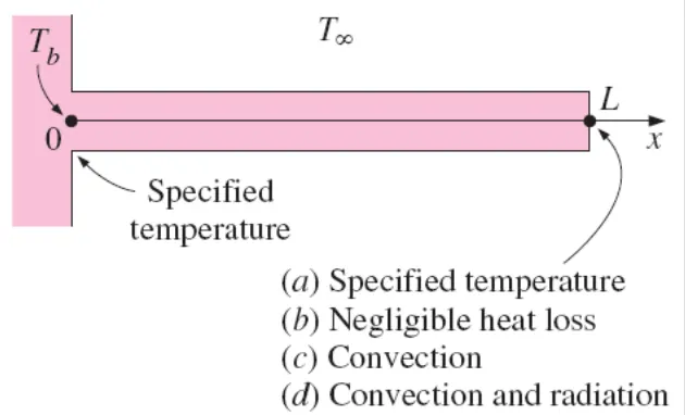
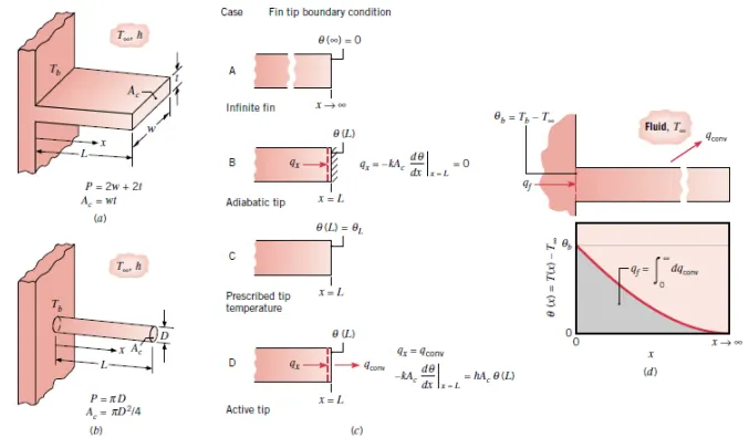
please refer the below photo for the Conduction and convection in a straight fin of uniform cross-sectional area. (a) Rectangular fin. (b) Pin fin. (c) Four common tip boundary conditions. (d) Temperature distribution for the infinite fin (x →∞)

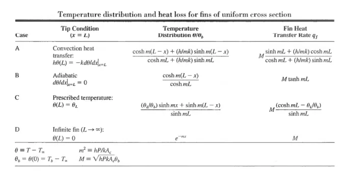
Please refer the below photo for the Temperature distribution, and loss heat of uniform sectional fins.

Fin Efficiency:

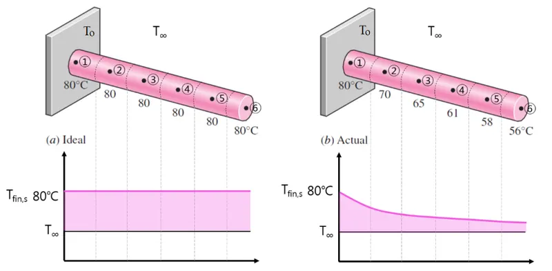
Temperature of a fin gradually drops along the length. In the limiting case of zero thermal resistance (k → ∞), the temperature of the fin will be uniform at the base value of To. The heat transfer from the fin will be maximized in this case: Qfin,max = hAfin(To − T∞)
Fin efficiency (ηfin) can be defined as:
ηfin =Qfin/Qfin,max=actual heat transfer rate from the fin/ideal heat transfer rate from the fin (if the entire fin were at base temperature)
Fin efficiency decreases with increasing fin length because of decrease in fin temperature with length.

Please refer the below photo for the Actual heat transfer rate and ideal heat transfer rate in the fins.

Fin effectiveness:

The performance of fins is judged on the basis of the enhancement in heat transfer relative to the no-fin case, and expressed in terms of the fin effectiveness.

Please refer the below photo for the heat transfer rate with fin and without fin.

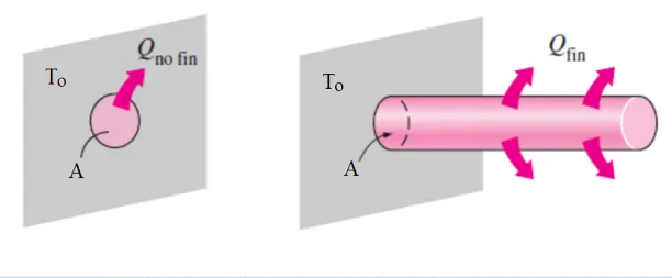
εfin =Qfin/Qno fin=heat transfer rate with fin/heat transfer rate without fin

If, εfin < 1 fin act as insulation
εfin = 1 fin does not affect heat transfer
εfin > 1 fin enhances heat transfer

Fins - Requirements:

1) Fins are generally used where convective heat transfer coefficient (h) values are relatively low. i.e., when air or gas is the medium and heat transfer is by natural convection.

2) Fin material should be of highly conductive materials.

3) Lateral surface area of the fin should be as high as possible.

4) The efficiency of most fins used in practice is above 90%.

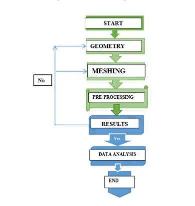
Please refer the below flow chart for the CFD work flow analysis of the steady-state conjugate heat transfer analysis on a model of a graphics card.

Geometry set-up:

We have to follow the following steps in the Geometry set-up.

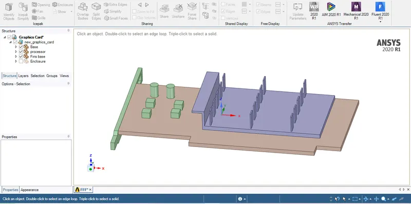
• Import the geometry and it consist of mainly 4 parts base, processer, fin and enclosure.
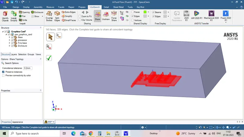
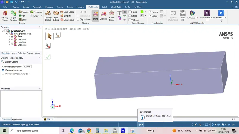
• Sharing the topology by using share tool which is available in the workbench.

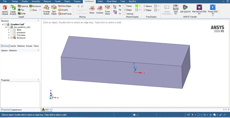
Please refer the below photo for the imported geometry for enclosure.

Please refer the below photo for the imported geometry for base and fin.

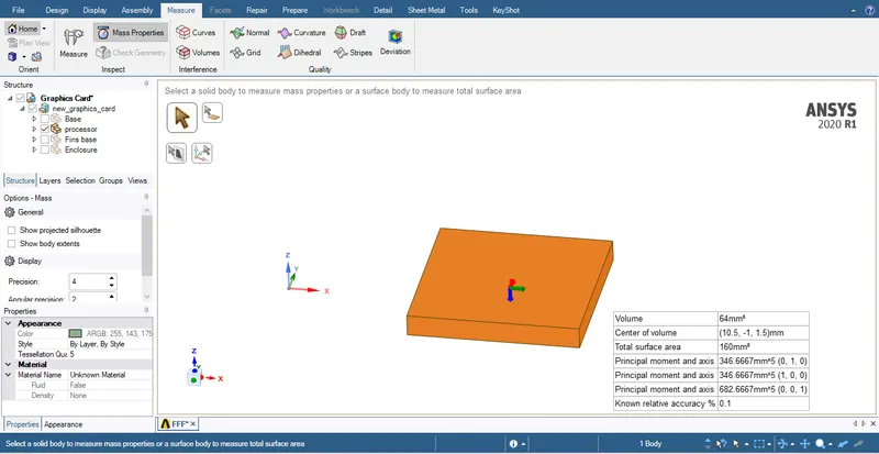
Please refer the below photo for the imported geometry for Processer and it's volume.

Please refer the below photo for the before sharing the topology.

Please refer the below photo for the after sharing the topology.

Meshing Set-up:

Following steps were followed in the Meshing Set-up.

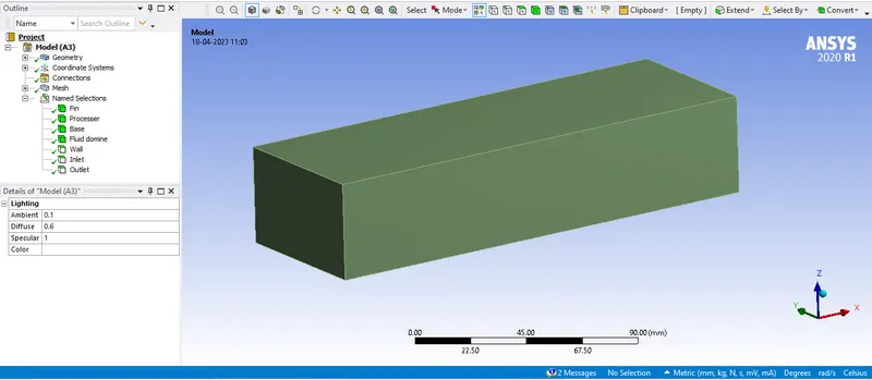
• Nomenclature of the graphics card model as inlet, outlet, Fin, processer, base and fluid domine.
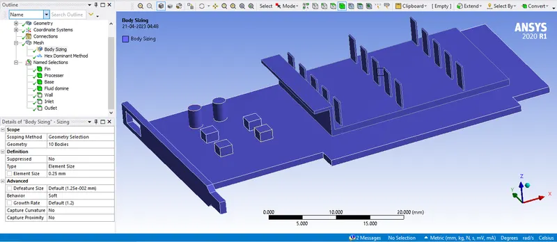
• Body sizing the fluid domine.
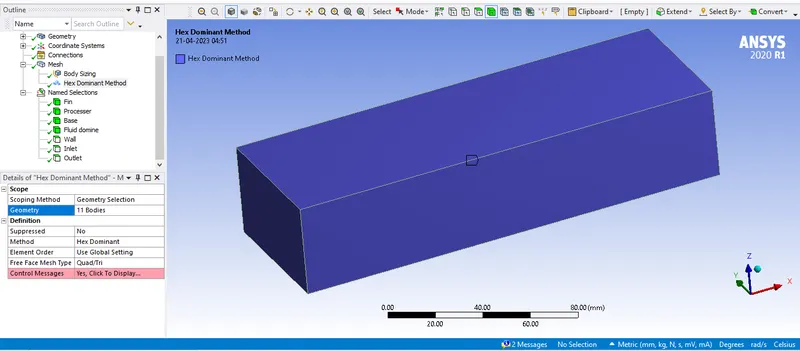
• Multizone Hexa Dominent method.

Please refer the below photos for the nomenclature of the graphics card model inlet, outlet, Fin, processer, base and fluid domine.

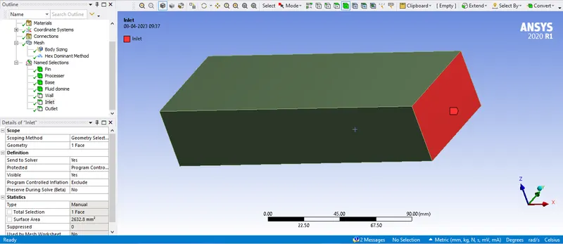
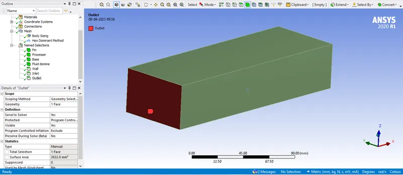
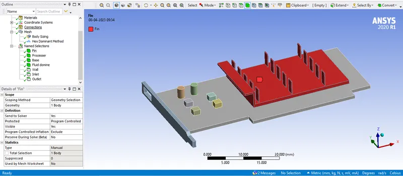
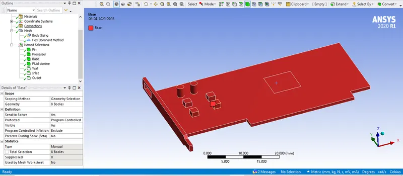
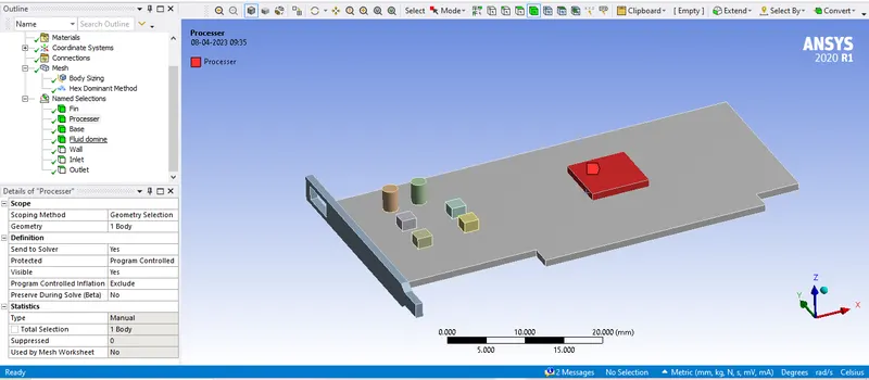
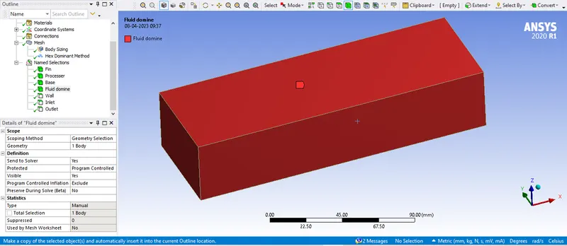
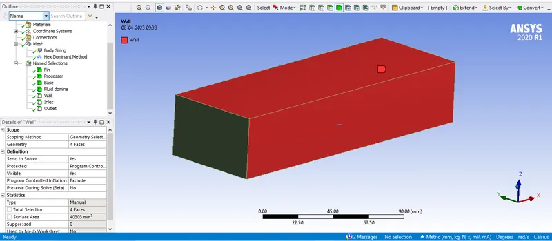
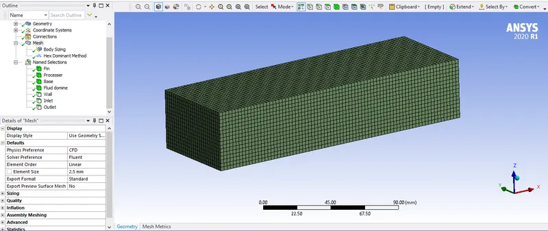
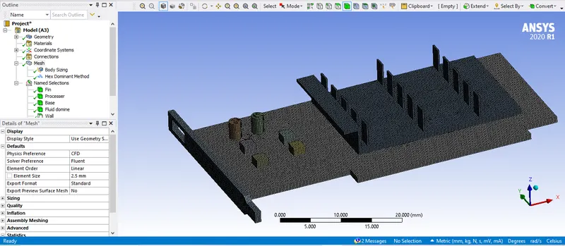
Please refer the below photo for the mesh element size applied i.e 2.5 mm.

Please refer the below photo for the Body sizing element size applied i.e 0.25 mm.

Please refer the below photo for the Multizone Hexa Dominent method applied

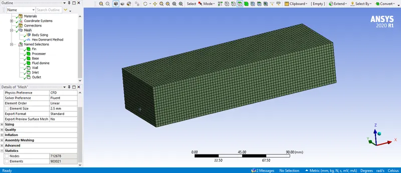
Please refer the below photo for the mesh element size 903021 nand nodes 712678 obtained.

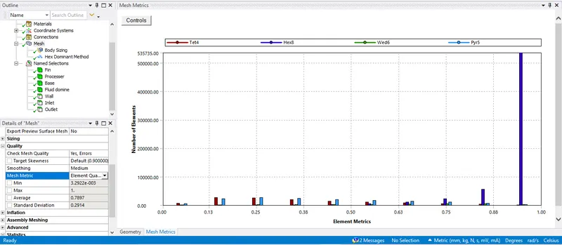
Please refer the below photo for the Element quality and the average value 0.7897 obtained.

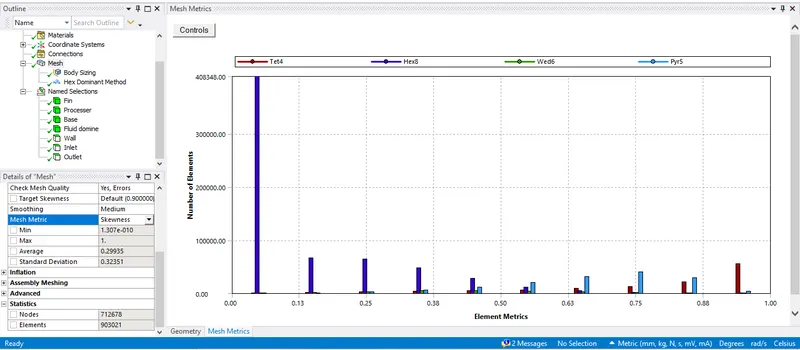
Please refer the below photo for the Skewness and the average value 0.29935 obtained.

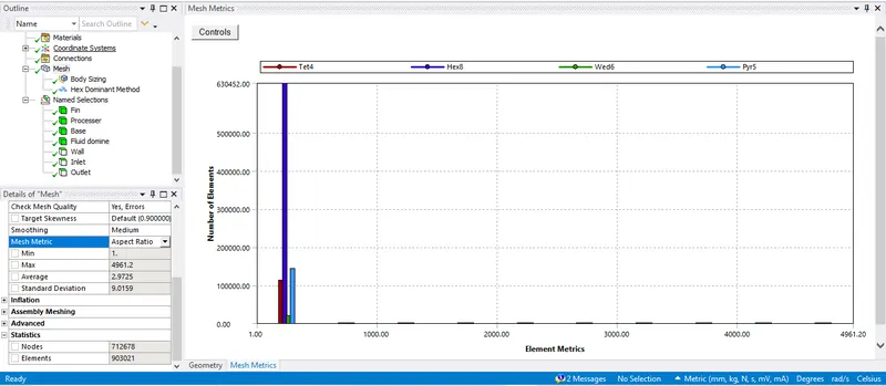
Please refer the below photo for the Aspect ratio and the average value 2.9725 obtained.

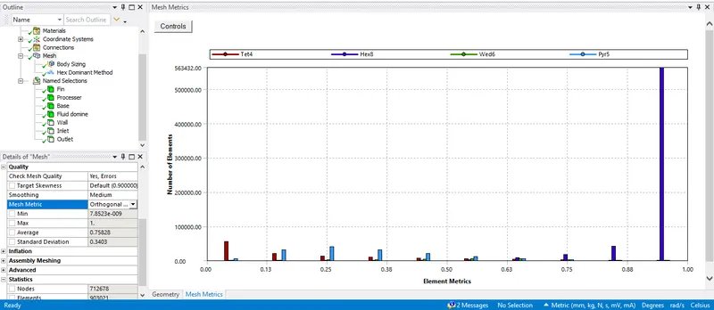
Please refer the below photo for the Ortogonal Quality and the average value 0.75828 obtained.

Fluent set up:

Please refer the below table for the fluent set-up inputs

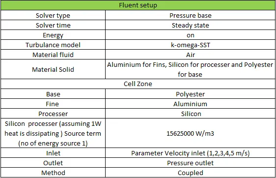
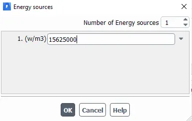
From the geometry set up it is observed that volume of the processer is 64 mm3.

We are assuming that the heat generated by the processer is 1 W (Watt).

The Energy discipated by the processer is given by the ratio of heat generated by the processer 1W to the volume of the processer 64 mm3.

By solving the above the Energy discipated by the processer is 15625000 W/m3.

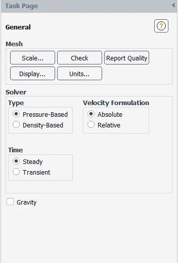
Please refer the below photo for the Solver type and time used and energy on.

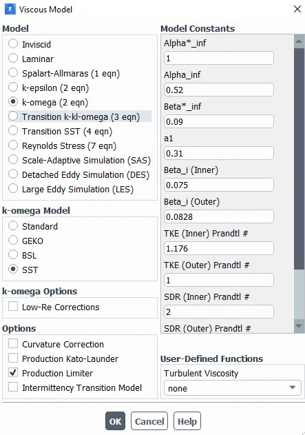
Please refer the below photo for the Turbulance model used.

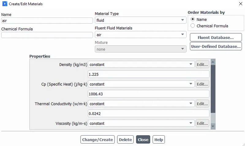
Please refer the below photo for the fluid Material Air applied and it's property.

Please refer the below photo for the solid Material Aluminium, Silicon and Polysteren applied and their property.

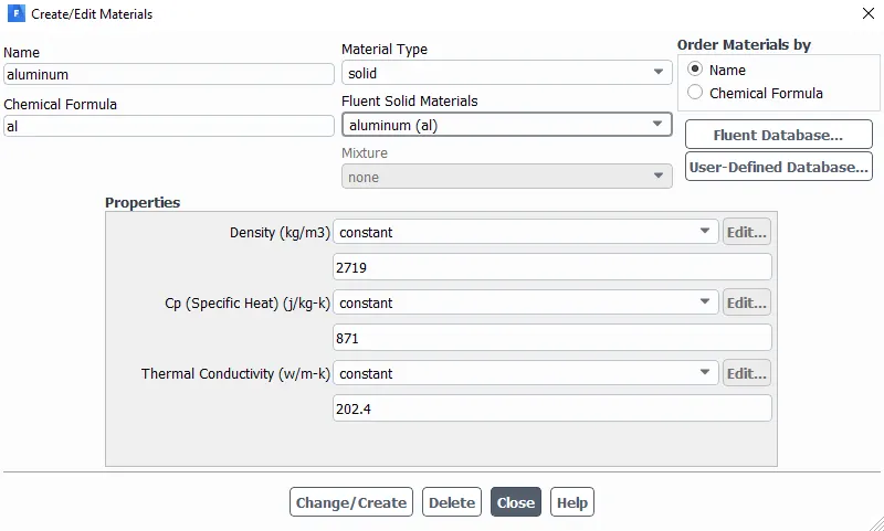
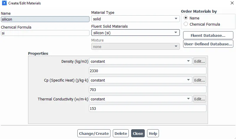
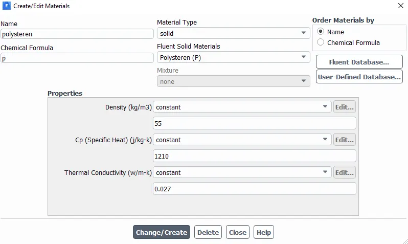
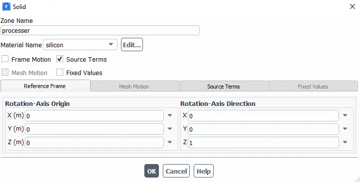
Apply the above defined material with respect to their cell zones as shown below.

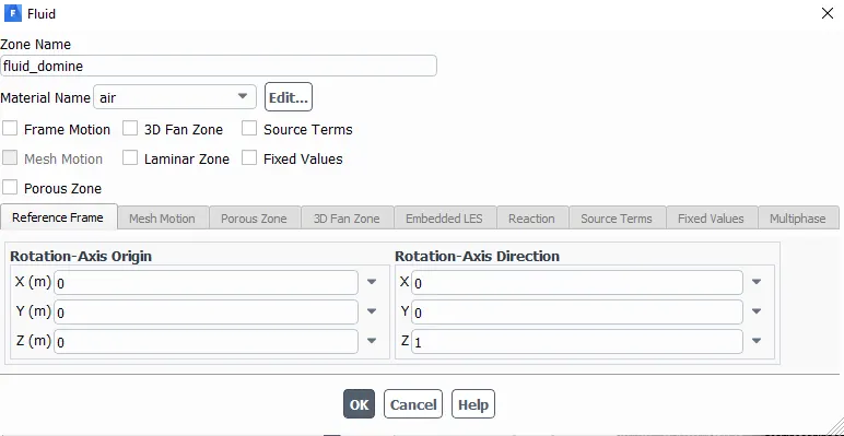
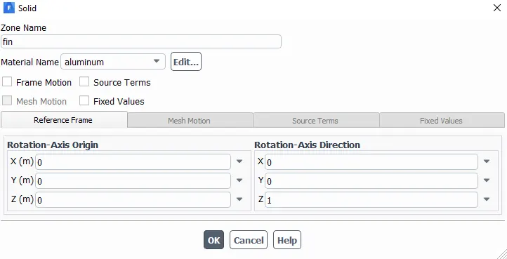
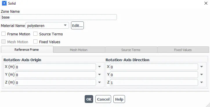
For the processer cell zone we have to enable the Energy source and give the Energy discipation rate of vovume as previously calculated 15625000 W/m3 as shown in the below.

Please refer the below photo for the inlet boundry conditions applied set velocity inlet as parameter for 5 velocity of 1 m/s, 2 m/s, 3m/s, 4 m/s and 5 m/s respectively.

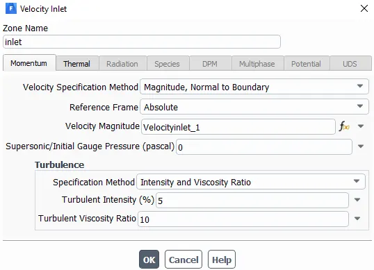
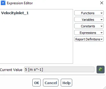
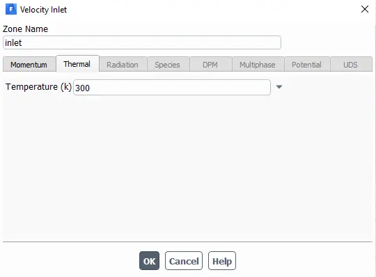
Report defination as shown below and seted as outlet parameter.

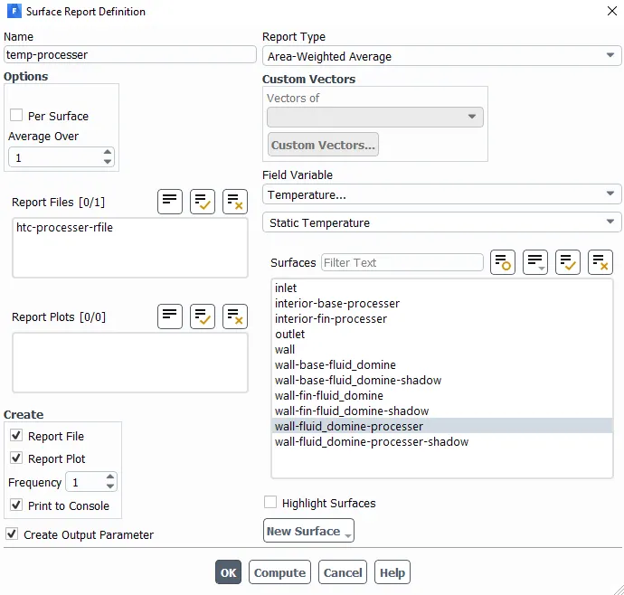
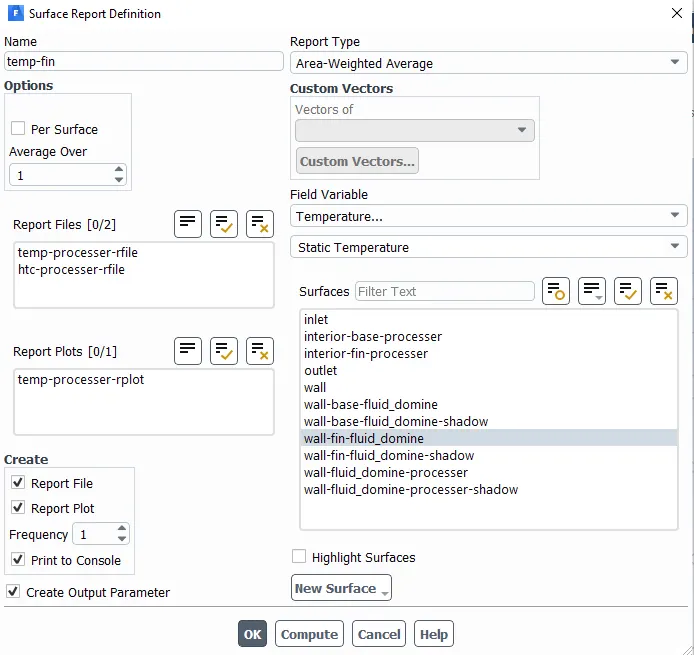
Hybrid Initialization has been done after the report defination and after run calculation has been done for the 300 itirations.

Result:

Case 1: Inlet velocity of 1 m/s

Please refer the below photo for the Residuals obtained.

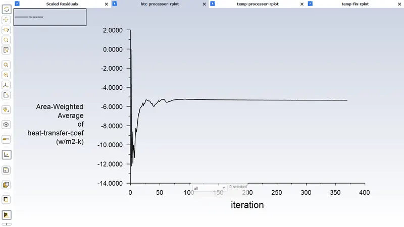
Please refer the below photo for the average htc-processer plot obtained.

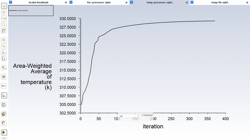
Please refer the below photo for the average Temperature-processer plot obtained.

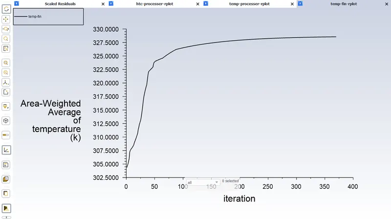
Please refer the below photo for the average Temperature-Fin plot obtained.

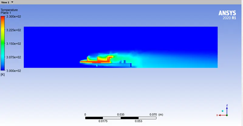
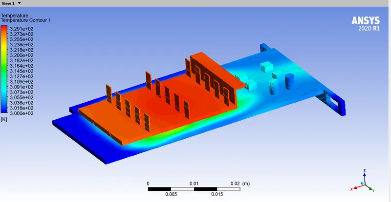
Please refer the below photo for the Temperature contour plot obtained with hotspot area.

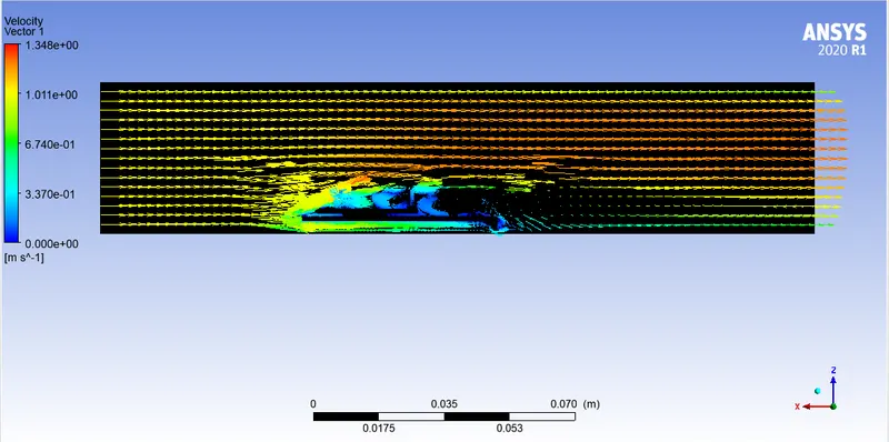
Please refer the below photo for the Velocity contour plot obtained.

Please refer the below photo for the results obtained.

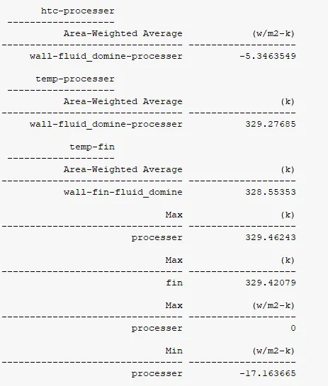
Case 2: Inlet velocity of 2 m/s

Please refer the below photo for the Residuals obtained.

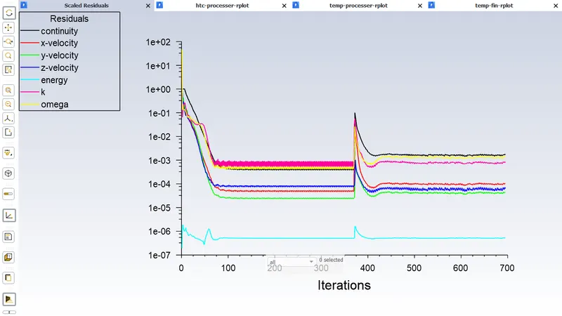
Please refer the below photo for the average htc-processer plot obtained.

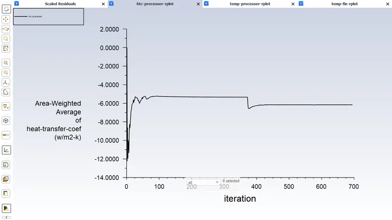
Please refer the below photo for the average Temperature-processer plot obtained.

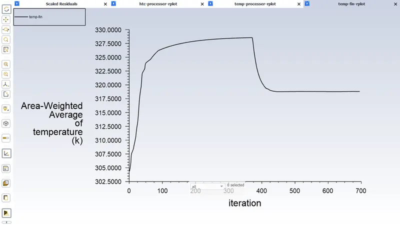
Please refer the below photo for the average Temperature-Fin plot obtained.

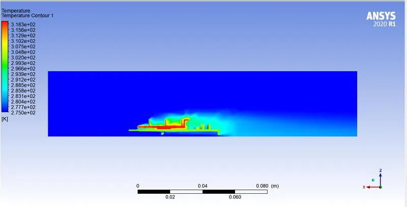
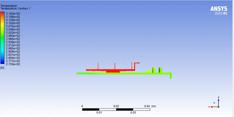
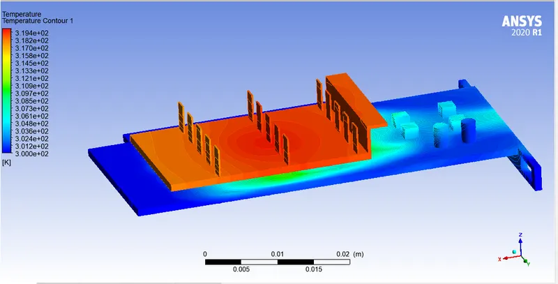
Please refer the below photo for the Temperature contour plot obtained with hotspot area.

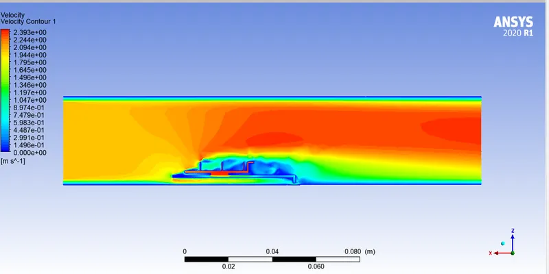
Please refer the below photo for the Velocity contour plot obtained.

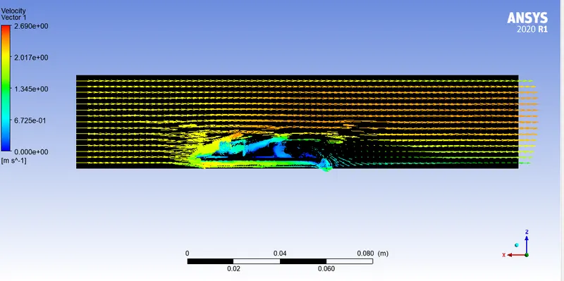
Please refer the below photo for the Velocity Vector plot obtained.

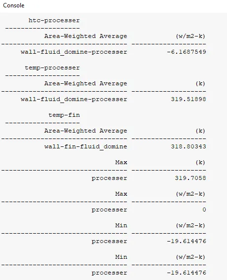
Please refer the below photo for the results obtained.

Case 3: Inlet velocity of 3 m/s

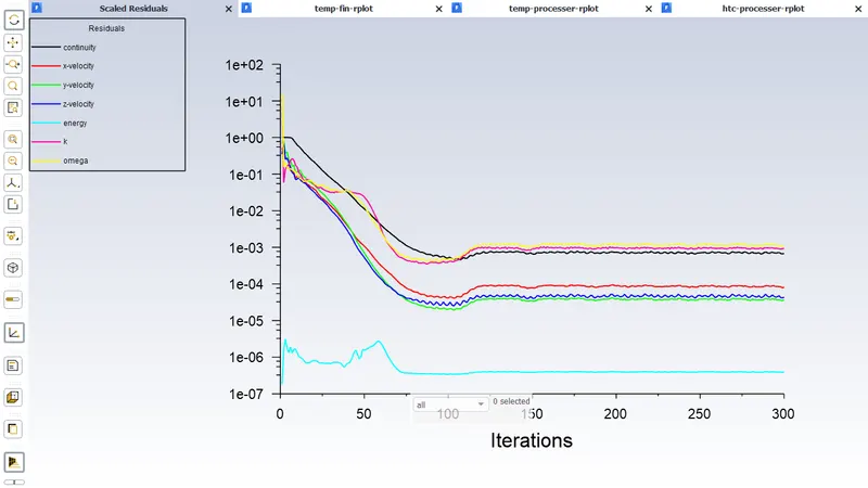
Please refer the below photo for the Residuals obtained.

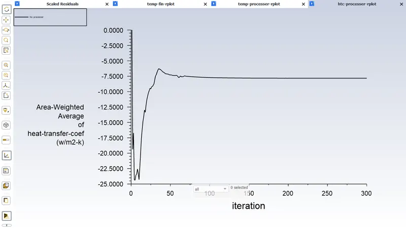
Please refer the below photo for the average htc-processer plot obtained.

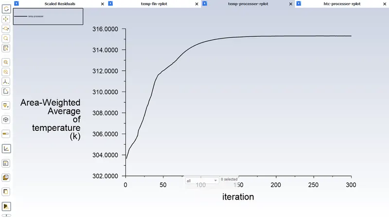
Please refer the below photo for the average Temperature-processer plot obtained.

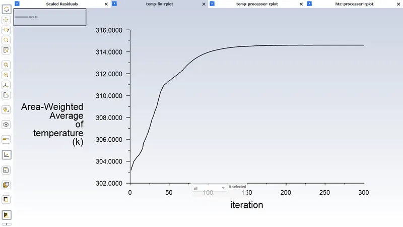
Please refer the below photo for the average Temperature-Fin plot obtained.

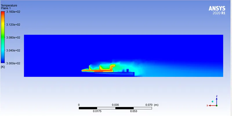
Please refer the below photo for the Temperature contour plot obtained with hotspot area.

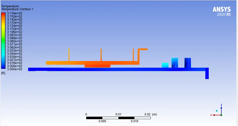
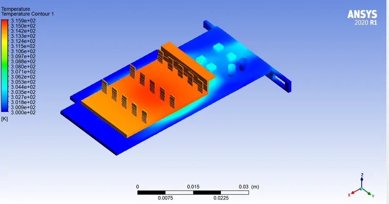
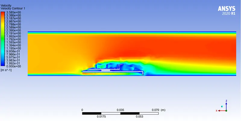
Please refer the below photo for the Velocity contour plot obtained.

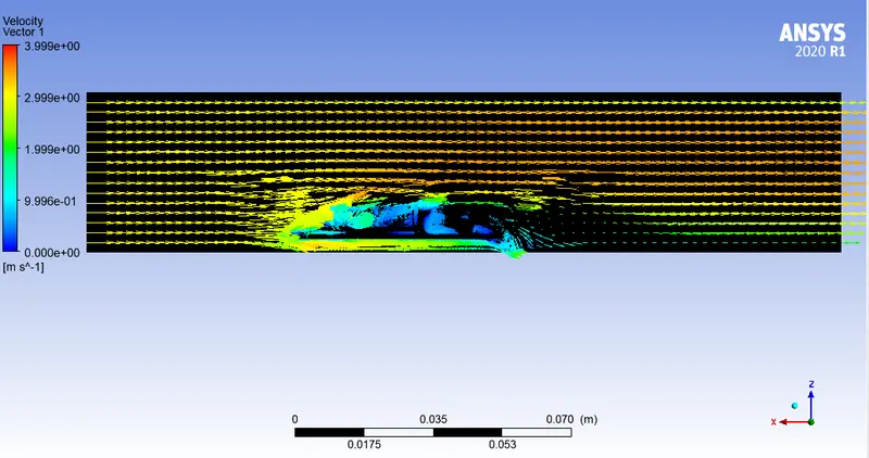
Please refer the below photo for the Velocity Vector plot obtained.

Please refer the below photo for the results obtained.

Case 4: Inlet velocity of 4 m/s

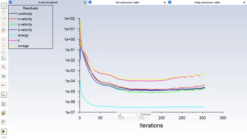
Please refer the below photo for the Residuals obtained.

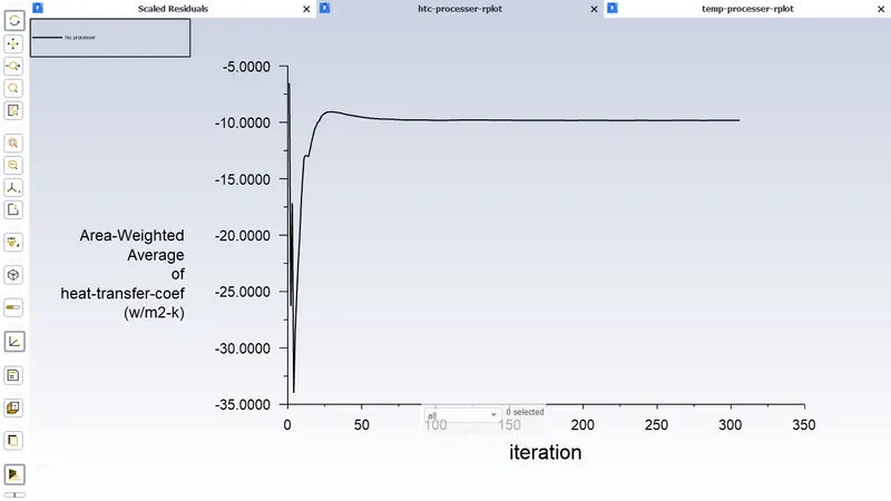
Please refer the below photo for the average htc-processer plot obtained.

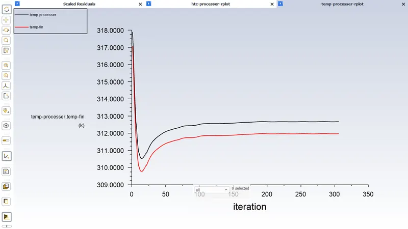
Please refer the below photo for the average Temperature-processer plot and average Temperature-Fin plot obtained.

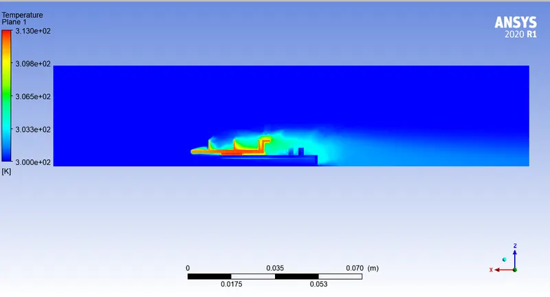
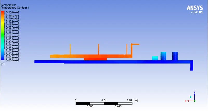
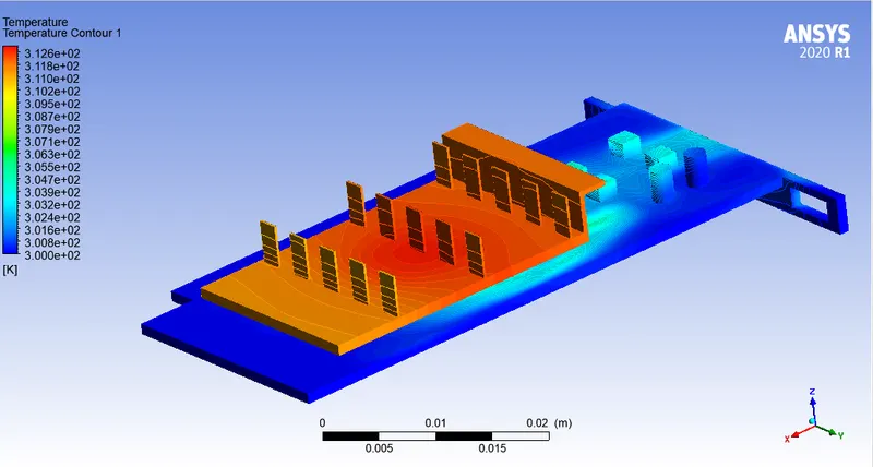
Please refer the below photo for the Temperature contour plot obtained with hotspot area.

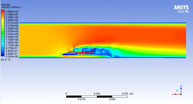
Please refer the below photo for the Velocity contour plot obtained.

Please refer the below photo for the Velocity Vector plot obtained.

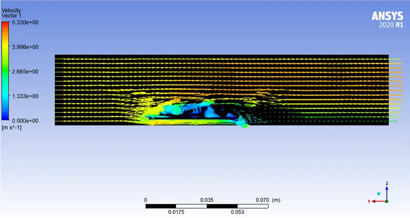
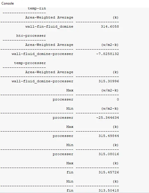
Please refer the below photo for the results obtained.

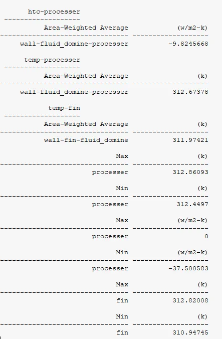
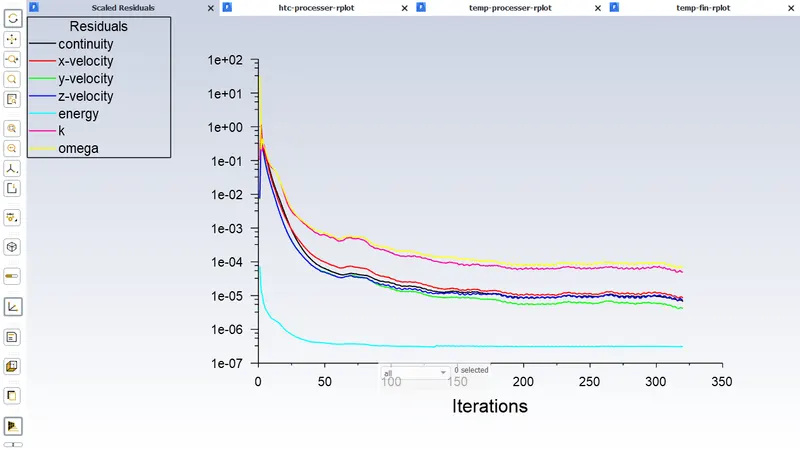
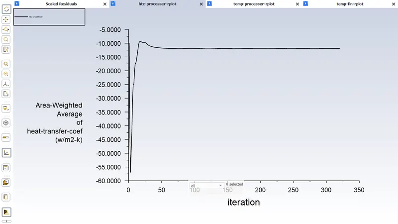
Case 5: Inlet velocity of 5 m/s

Please refer the below photo for the Residuals obtained.

Please refer the below photo for the average htc-processer plot obtained.

Please refer the below photo for the average Temperature-processer plot obtained.

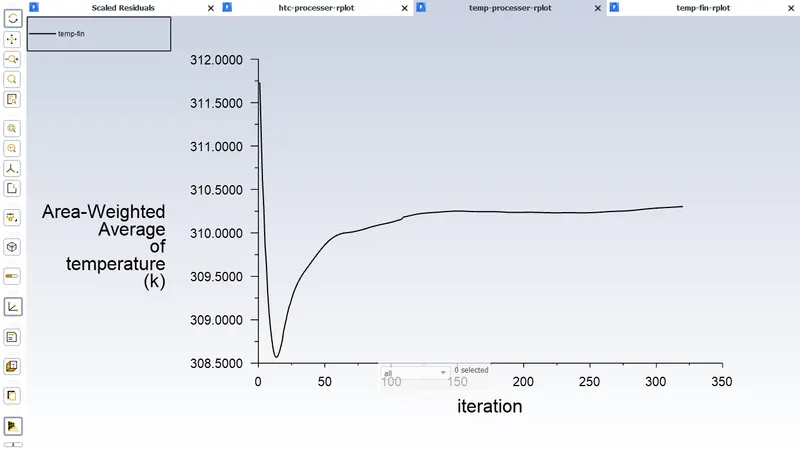
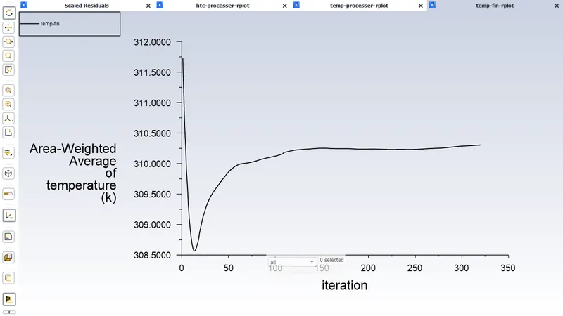
Please refer the below photo for the average Temperature-Fin plot obtained.

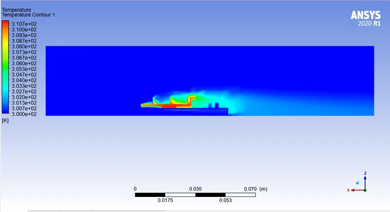
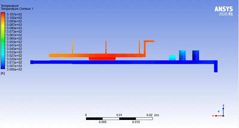
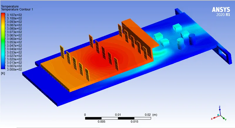
Please refer the below photo for the Temperature contour plot obtained with hotspot area.

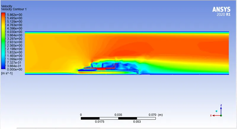
Please refer the below photo for the Velocity contour plot obtained.

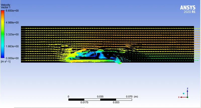
Please refer the below photo for the Velocity Vector plot obtained.

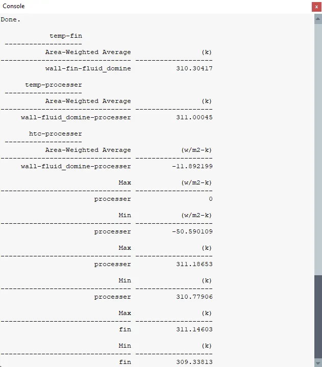
Please refer the below photo for the results obtained.

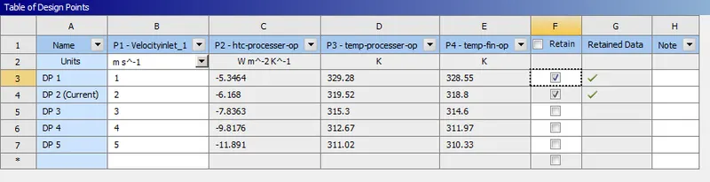
Pleasde refer the below photo for the overview of inlet and outlet parameters obtained.

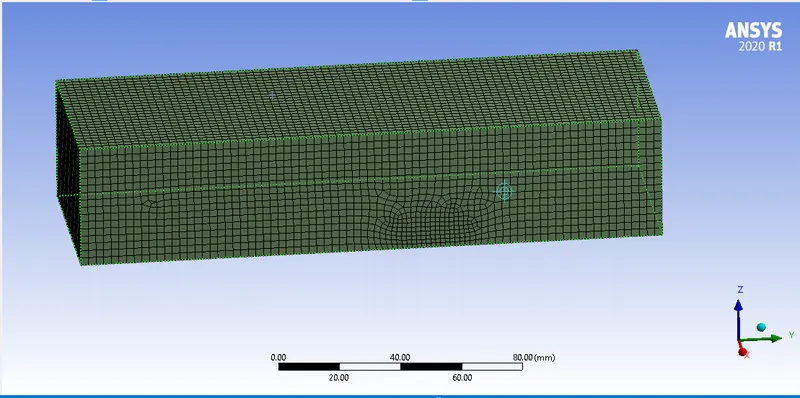
Case 6: Inlet velocity of 1 m/s with change in the geometry of inlet and outlet in X direction to Y direction. All the other condition remains same as in the above cases.

Please refer the below photo for the geometry change.

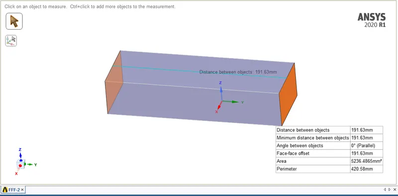
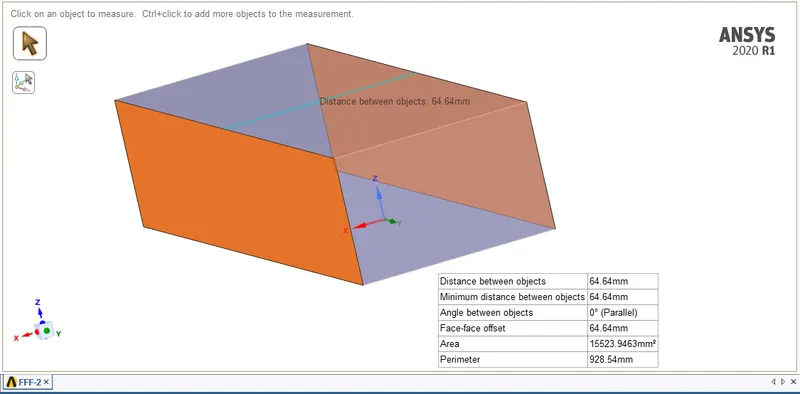
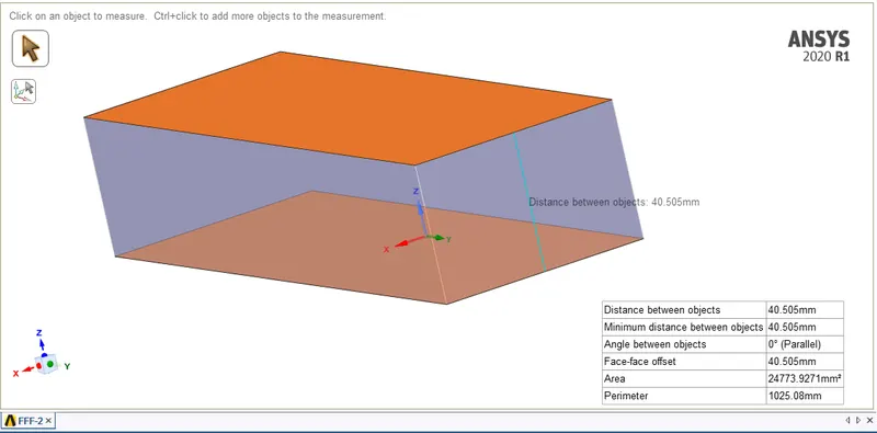
Graphicd card is 85 mm away from the outlet and 50 mm away from the inlet length and 1 mm bottom clearance and 30 mm away up to top in thickness.

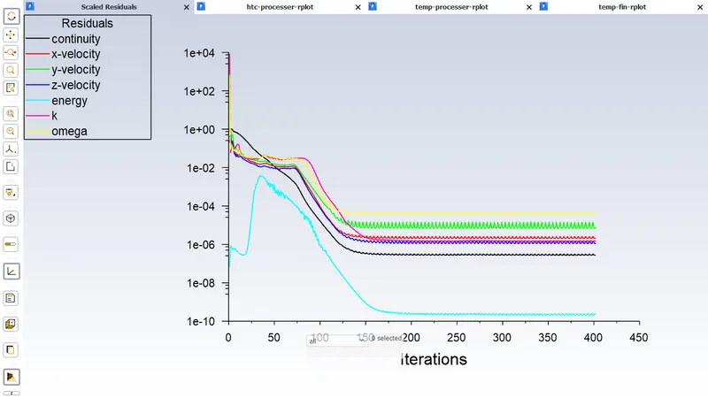
Please refer the below photo for the Residuals obtained.

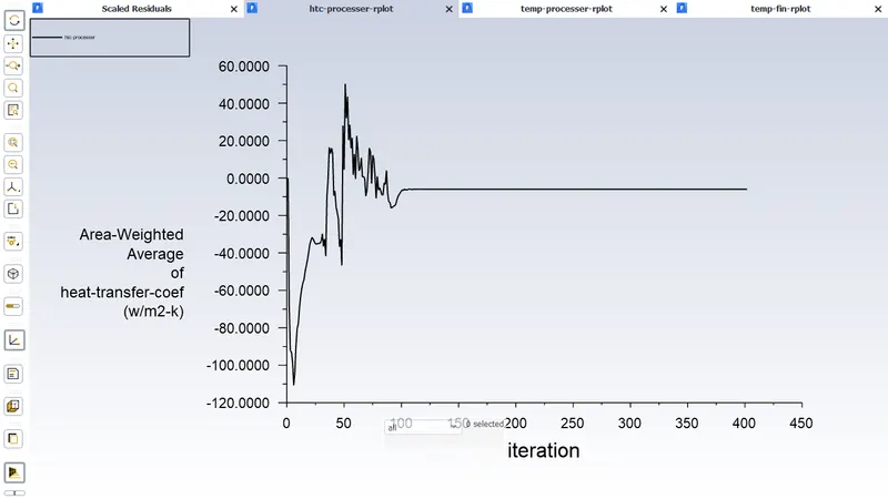
Please refer the below photo for the average htc-processer plot obtained.

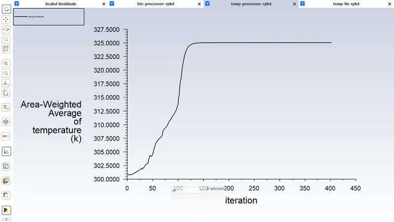
Please refer the below photo for the average Temperature-processer plot obtained.

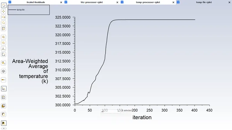
Please refer the below photo for the average Temperature-Fin plot obtained.

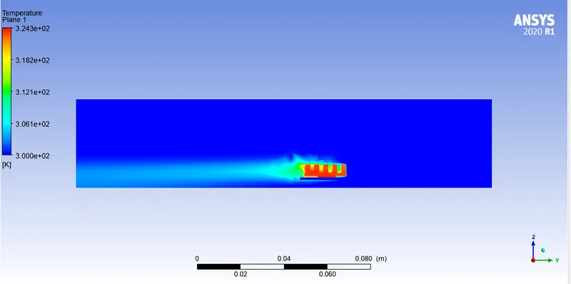
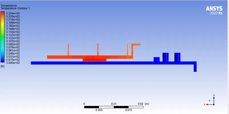
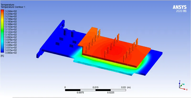
Please refer the below photo for the Temperature contour plot obtained with hotspot area.

Please refer the below photo for the Velocity contour plot obtained.

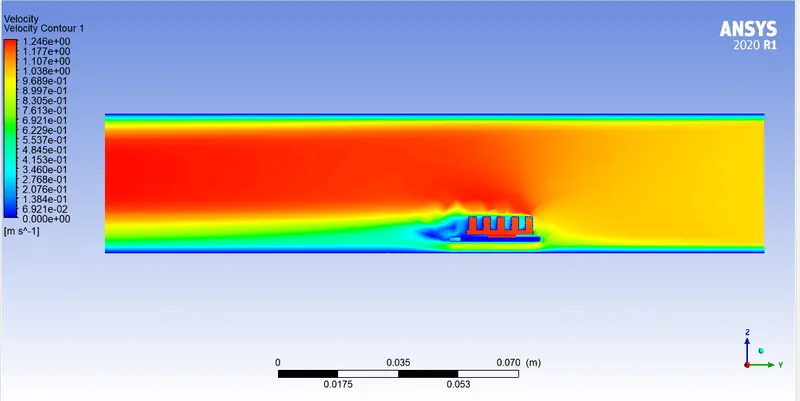
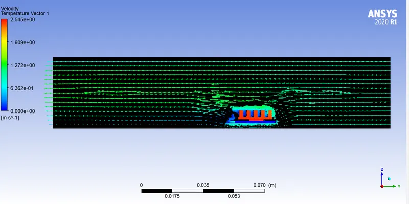
Please refer the below photo for the Velocity Vector plot obtained.

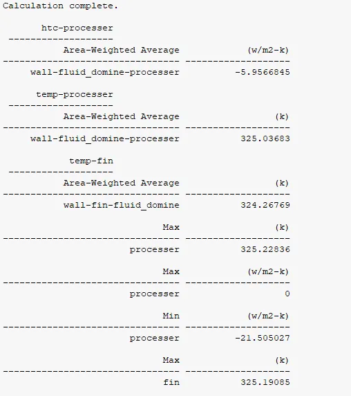
Please refer the below photo for the results obtained.

Please refer the below table for the final results obtained.

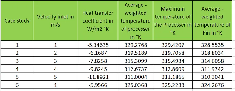
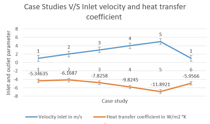
Here heat transfer coefficient -ve signe indicates heat is loss or discipation by the system or Processer. From the above table it is clear that as we increase the velocity the heat loss or discipation rate also increases.

Please refer the below graph of case studies and Inlet velocity and heat transfer coefficient. From the graph it is observed that the velocity increases the heat loss or discipation rate also increases except case 6.

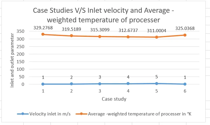
Please refer the below graph of case studies and Inlet velocity and Average -weighted temperature of processer. From the graph it is observed that the velocity increases the Average -weighted temperature of processer decreases except case 6

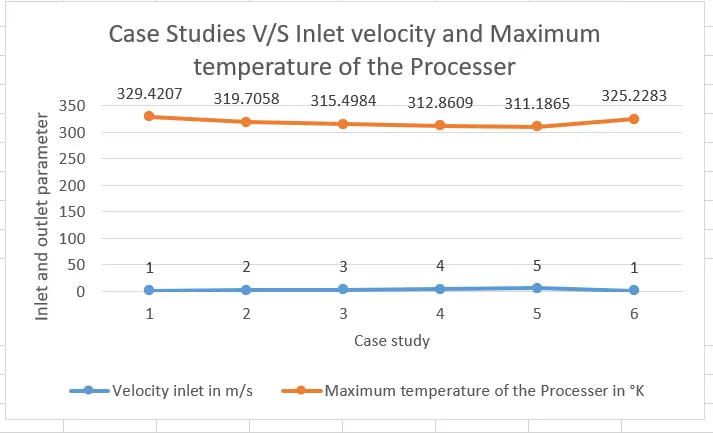
Please refer the below graph of case studies and Inlet velocity and Maximum temperature of the Processer. From the graph it is observed that the velocity increases the Maximum temperature of the Processer decreases except case 6

Please refer the below graph of case studies and Inlet velocity and Average -weighted temperature of Fin. From the graph it is observed that the velocity increases Average -weighted temperature of Fin decreases except case 6.

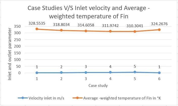
It is concluded that at higher velocity the heat descipation rate is more and the temperature of the processer and fin reduces.

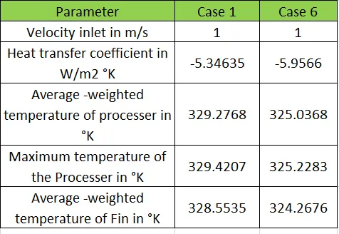
Comparision of Case 1 to Case 6:

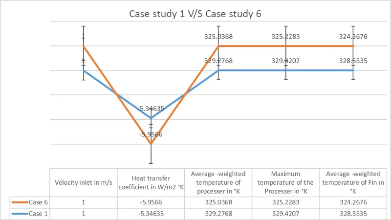
By comparing the case study 1 and 6 it is concluded that the Case 6 gives better results than case 1

Please refer the below table of comparision of Case 1 and Case 6.

Please refer the below graph of comparision of Case 1 and Case 6.