Week 2 - Flow over a Cylinder.

AIM:

Simulate the flow over a cylinder and explain the phenomenon of Karman vortex street.

PART-I

1. Simulate the flow with the steady and unsteady case and calculate the Strouhal Number for Re= 100.

PART-II

1. Calculate the coefficient of drag and lift over a cylinder by setting the Reynolds number to 10,100,1000,10000 & 100000. (Run with steady solver)
2. Discuss the effect of Reynolds number on the coefficient of drag. [ Results should be validated with any standard literature and error should be within 5 %]

OBJECTIVE:

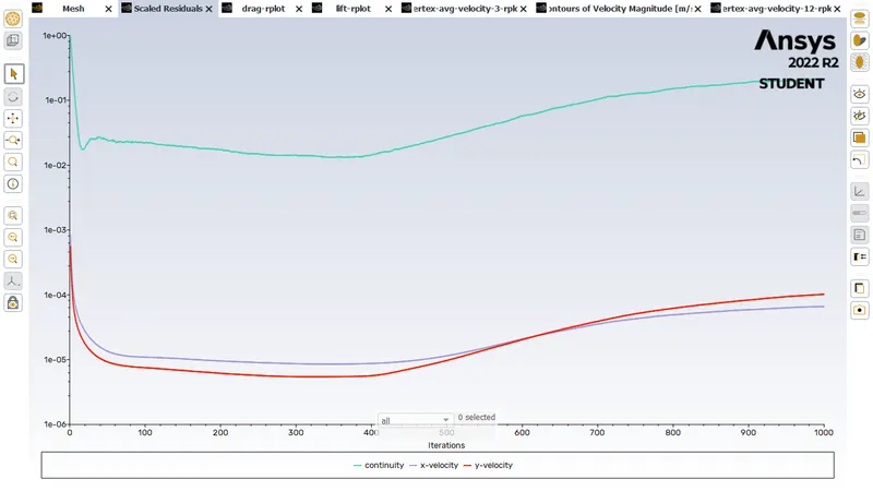
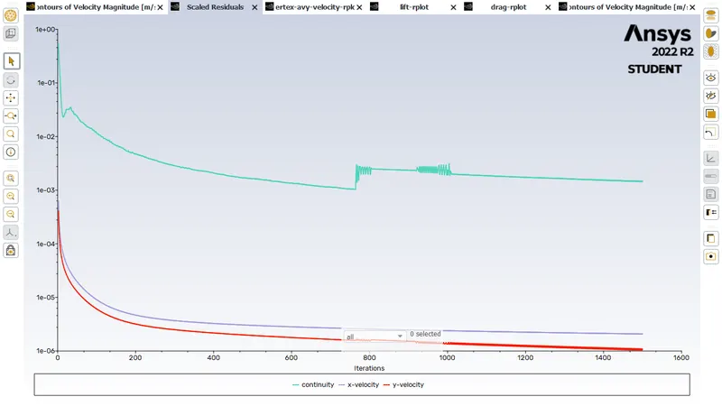
• In both approaches, show that the flow has converged. That is, what quantities or plots need to be looked at to determine that the flow has converged?
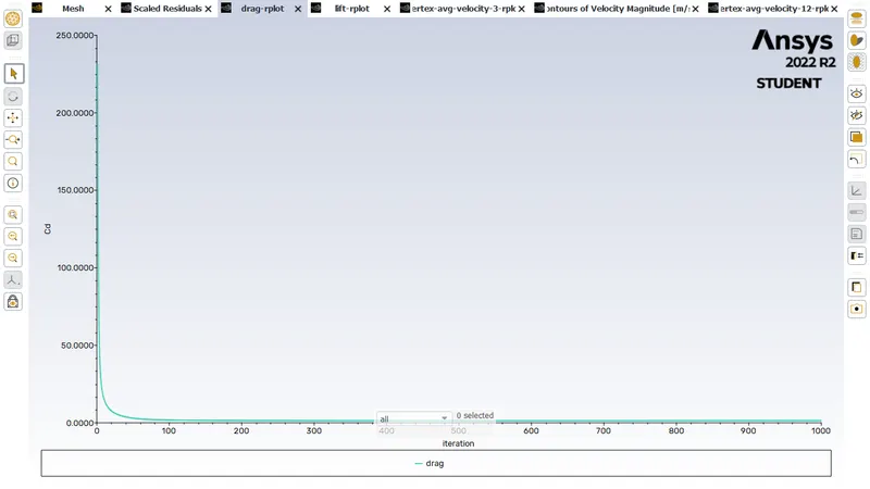
• Plots of the coefficient of drag and lift.
• Plots to show vortex shedding behind the cylinder.
• Mention the referred material (Reference Paper or Fluid Mechanics Textbook) at the end of the challenge submission page.

THEORY:

Reynolds number:

Reynolds number is a dimensionless quantity that is used to determine the type of flow pattern as laminar or turbulent while flowing through a pipe. Reynolds number is defined by the ratio of inertial forces to that of viscous forces.

It is given by`R=(ρvD)/μ`

Where,R is the Reynolds number

ρ is the density of the fluid (kg/m³)

V is the velocity of flow (m/s)

D is the pipe diameter (m)

μ is the viscosity of the fluid (kg/m-s)

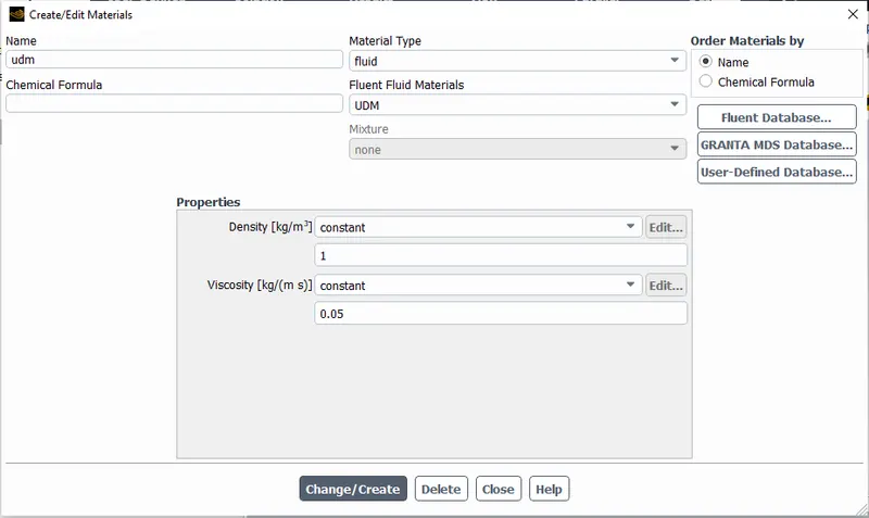
For the Re 10, 100, 1000, 10000 and 100000 and constant density of 1 kg/m3, diameter of 2 m and viscosity of 0.05 kg/m-s we have the following velocity respectively.

Velocity is given by `v = (R⁡μ)/(ρD)`

`v=(R 0.05)/(1 X 2)`

Generalized equation is V=Re*0.025

For Re10, V=10*0.025=0.25 m/s --------------------------------i

For Re100, V=100*0.025=2.5 m/s -------------------------------ii

For Re1000, V=1000*0.025=25 m/s ----------------------------iii

For Re10000, V=10000*0.025=250 m/s ------------------------iv

For Re100000, V=100000*0.025=2500 m/s -------------------v

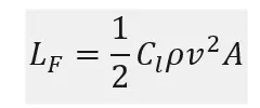
Lift Force:

The force which is acting perpendicular to the object or body of motion is called Lift force.

It is given by the equation

Lift coefficient equation is given by

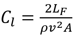
LF denotes lift force

ρ denotes density (kg/m³)

A denotes the frontal area (m²)

v denotes velocity (m/s)

C_l denotes lift coefficient

Lift coefficient: The lift coefficient expresses the ratio of the lift force to the force produced by the dynamic pressure times the area.

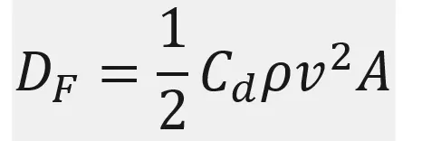
Drag Force:

Drag force is a resistance force which is acting opposite towards the motion of the object which is moving submerged in a certain fluid. drag force can also be defined as the force that counterattacks or resists the motion of a body in a fluid. The fundamental nature of drag force is to act in the opposite direction of the flow velocity. The value of drag force is directly proportional to the density of fluid, square of the velocity, cross-section area and the drag coefficient. For smooth surfaces the drag force is less and for flat plates the drag force is high.

It is given by the equation

Drag Coefficient equation is given by

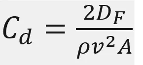
DF denotes drag force

ρ denotes density (kg/m³)

A denotes the frontal area (m²)

v denotes velocity (m/s)

C_d denotes drag coefficient

Drag Coefficient: When an object moves through a fluid, then to compute its resistance, the coefficient used is known as the Drag coefficient, denoted by C_d. The coefficient of drag is dimensionless, which is helpful in calculating aerodynamic drag and the impact of shape, inclination, and conditions of flow in aerodynamics.

Von-Karman Vertex Street:

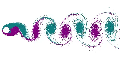
Von-Karman Vertex Street is a repeating pattern of swirling vortices, caused by a process known as vortex shedding, which is responsible for the unsteady separation of flow of a fluid around blunt bodies.

These vortices produce a sinusoidal force acting on the body perpendicular to the flow. Please refer the below animation for the visual understand of Von-Karman Vertex Street.

Strouhal number:

The Strouhal number is defined as St = ꞷD/U, where ꞷ is the vortex shedding frequency (or the Strouhal frequency) of a body at rest, D is the diameter of the circular cylinder and U is the velocity of the ambient flow.

The Strouhal Number can be important when analysing unsteady, oscillating flow problems. The Strouhal Number represents a measure of the ratio of the inertial forces due to the unsteadiness of the flow or local acceleration to the inertial forces due to changes in velocity from one point to another in the flow field.

Boundary layer:

Boundary layer is a region around the body within it viscous forces are significant. A thin layer of fluid is formed close to the solid surface where the gradient in velocity or any scalar is significant. This thin region is called as boundary layer.

Boundary layers are thin, viscosity-dominant regions that form along the surface of a solid body as a fluid flows past it.

The gradient in the mean velocity and temperature is steep normal to the wall.

Inflation layer:

The Inflation function in ANSYS Fluent allows to stack elements and cells in a unique way that is often only possible at their boundaries. An inflating layer can be created by trapping the normal gradient close to no-slip barriers. Only thin elements and a small number of elements can be used to achieve this.

The inflation layer control is designed to create thin elements that can capture the normal gradient with minimal elements; use inflation layers to correctly capture the velocity and temperature gradients near no-slip walls.

In this challenge we are using the 5mm inflation layer.

Flow separator:

When the fluid is forced to flow over a curved surface at high velocity a fluid flows in the front portion of the curved surface with no problem, but it is difficult to the surface on the back side, at sufficient high velocity the fluid streams detach itself from the surface of the body this is called flow separation.

The location of separation point depends on several factors such as Reynolds number, the surface roughness and the level of fluctuations. It is usually difficult to predict the exactly where the separation will occur unless there is a sharp corner, or abrupt changes in the shape of the solid surface.

GEOMETRY OF THE MODEL:

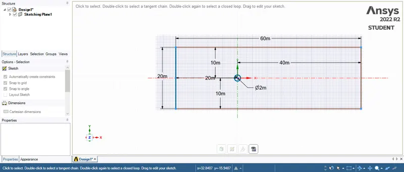
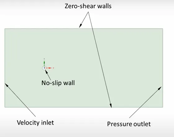
As we are using the 2D simulation we have to creat 20mX60m rectangle and the circle of 2m Dia which is 20m away from the front and 10m above and below as shown in the below diagram.

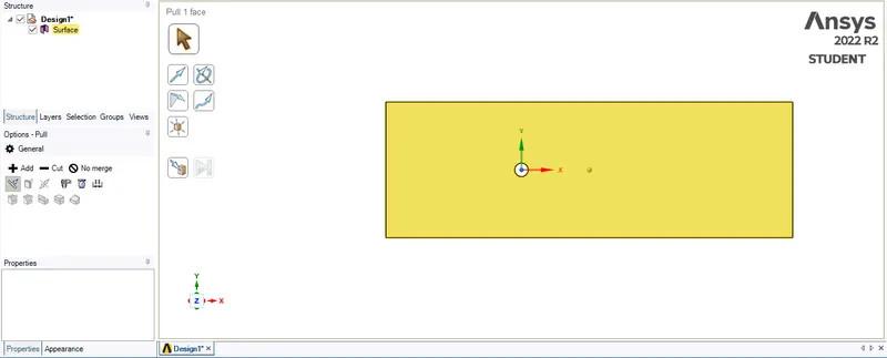
After the surface created it will look like the below diagram.

MESH PREPARATION:

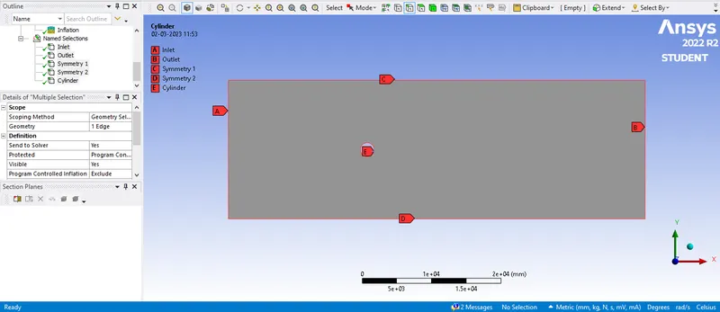
Nomenclature of the geometry has been done please refer the below photo of it.

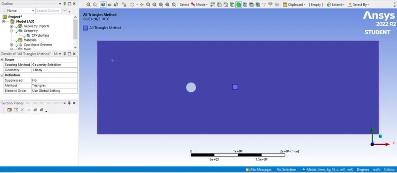
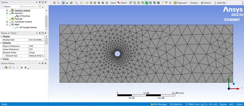
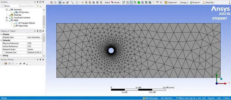
Please refer the below photo for the triangle type mesh obtained.

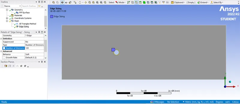
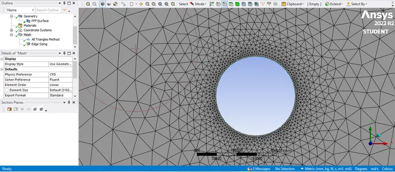
Please refer the below photo for edge sizeing the mesh for 120 obtained.

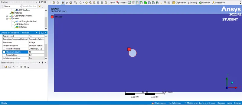
Please refer the below photo for the inflamation of 3mm and 15 layers obtained.

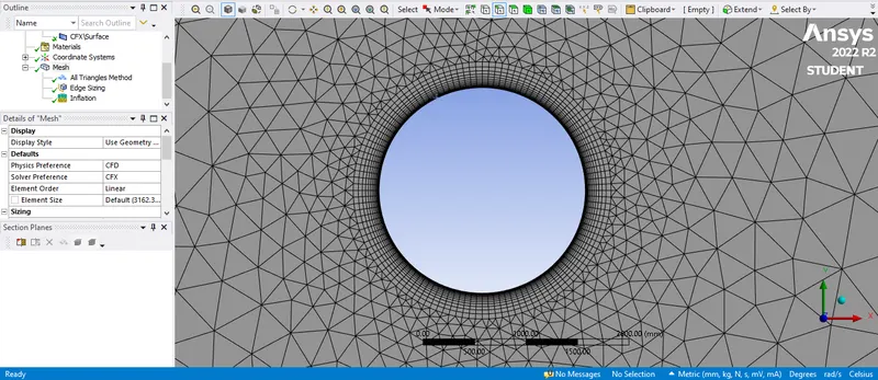
Please refer the below photo for the 100mm mesh and obtained .

SETUP SOLVER PREPARATION:

Please refer the below photo for the solver type used for both study and unstudy flow respectively.

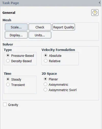
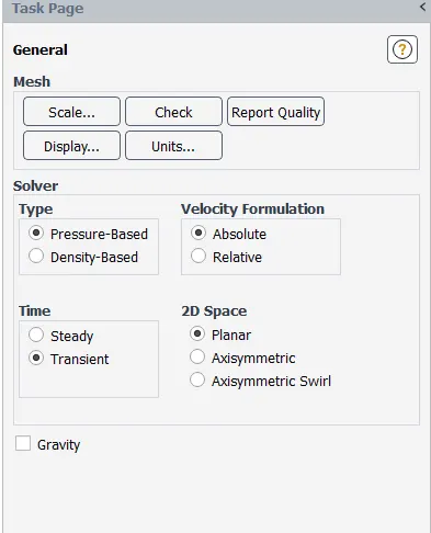
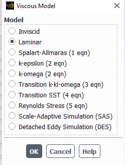
Please refer the below photo for the laminar flow model applied.

Please refer the below photo for air as fluid with their properties.

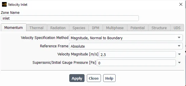
Please refer the below photo for the Velocity inlet it will change accoring the Reynolds number as calculatrd above.

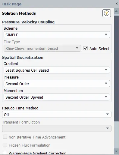
Please refer the below photo for the solution SIMPLE method applied.

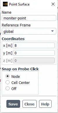
Please refer the below photo for the monitor point created at 8 m away from the cylinder wall.

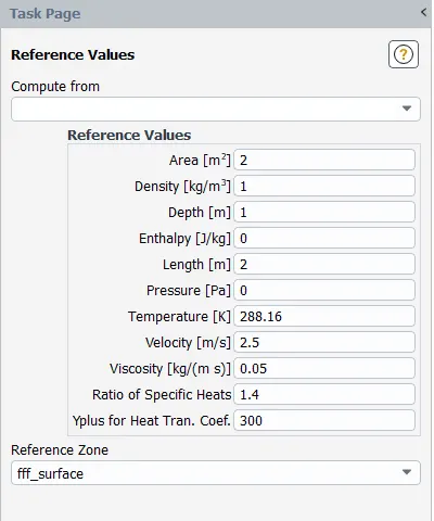
Please refer the below photo for the Reference Value entered velocity vary according the Reynolds number.

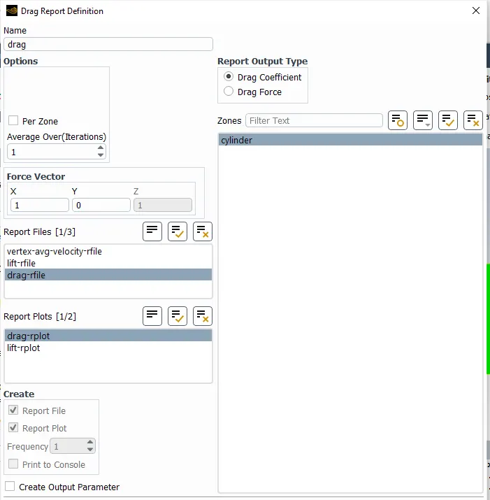
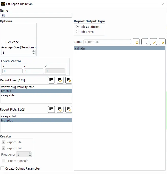
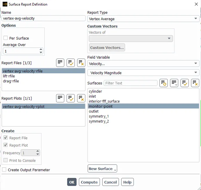
Please refer the below photo for the Drag, Lift, Vertex-Avg-Velocity and Velocity contour plot inputs respectively

.

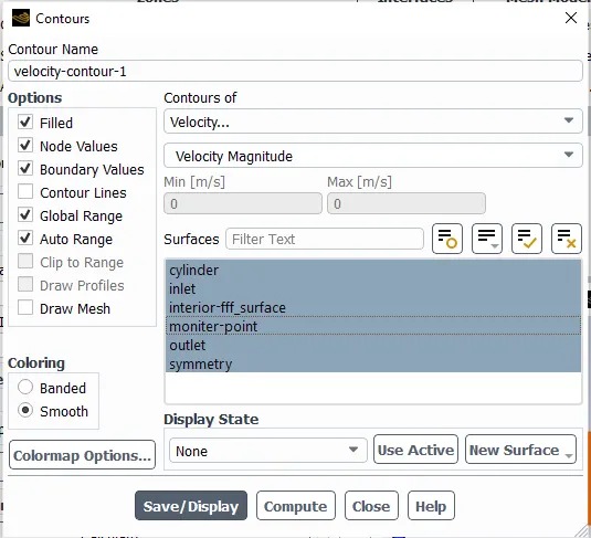
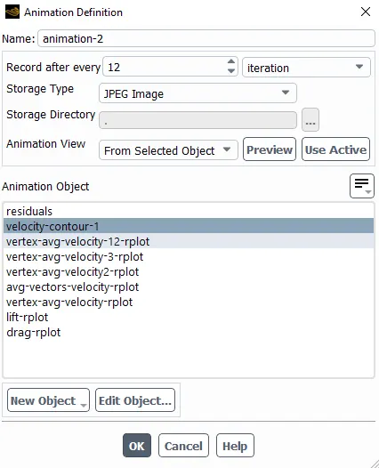
Please refer the below photo for the animation file input given.

PART I RESULTS:

For study flow for the Reynolds number 100.

Please refer the below photo for the Residuals obtained.

Please refer the below photo for the Drag plot obtained.

Please refer the below photo for the Lift plot obtained.

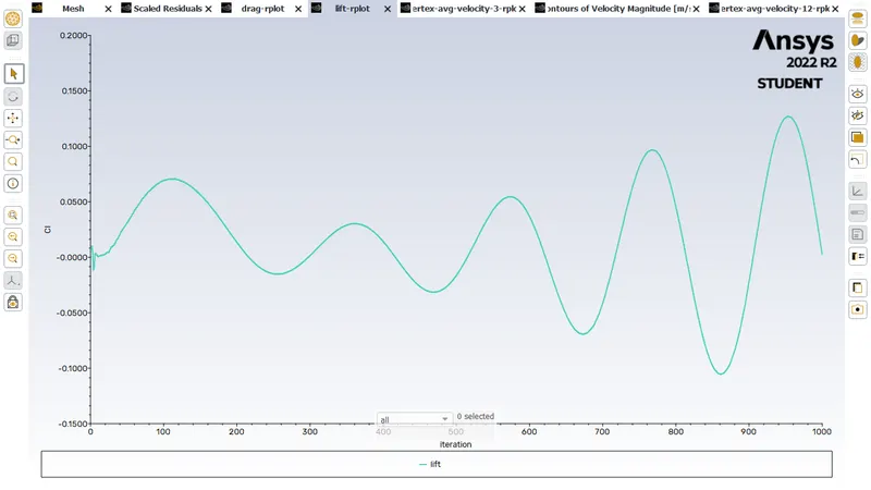
Please refer the below photo for the Vertex-Avg-Velocity plot obtained.

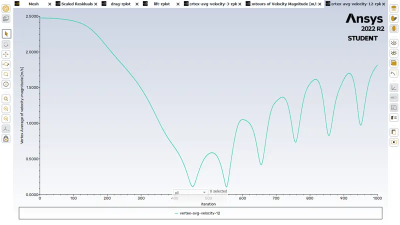
Please refer the below photo and animation for the Velocity contour plot obtained.

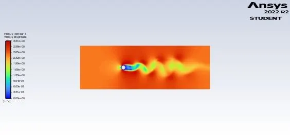
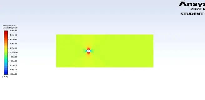
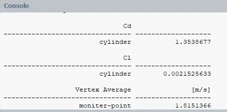
Please refer the below photo for the values obtained for the above plots.

Please refer the below photo for the Magnitude VS Strouhal number obtained.

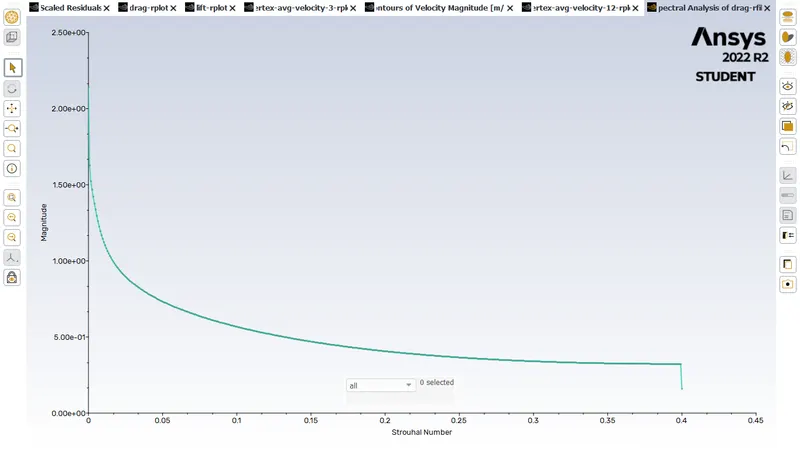
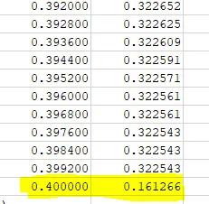
Strouhal number obtained is 0.161266 as highlighted in the above photo from the graph values.

For Unstudy/Transient flow for the Reynolds number 100.

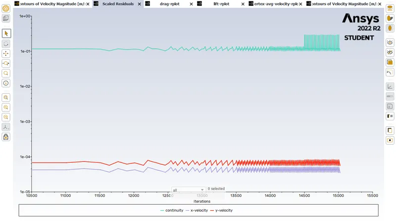
Please refer the below photo for the Residuals obtained.

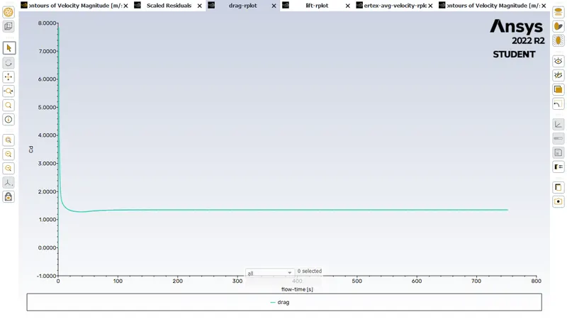
Please refer the below photo for the Drag plot obtained.

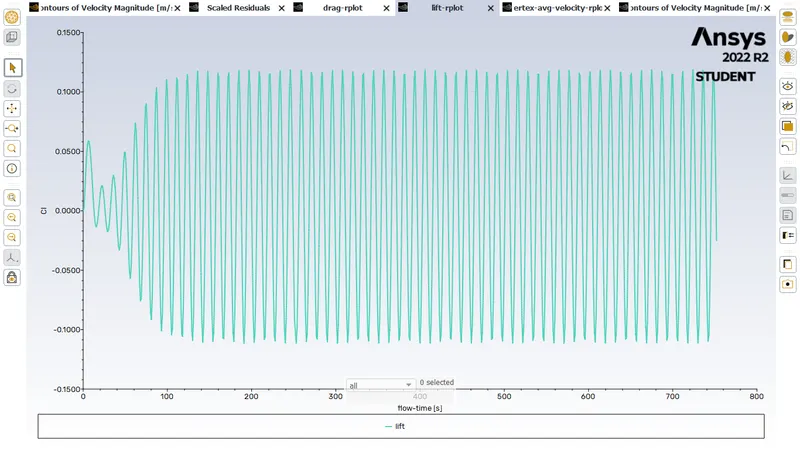
Please refer the below photo for the Lift plot obtained.

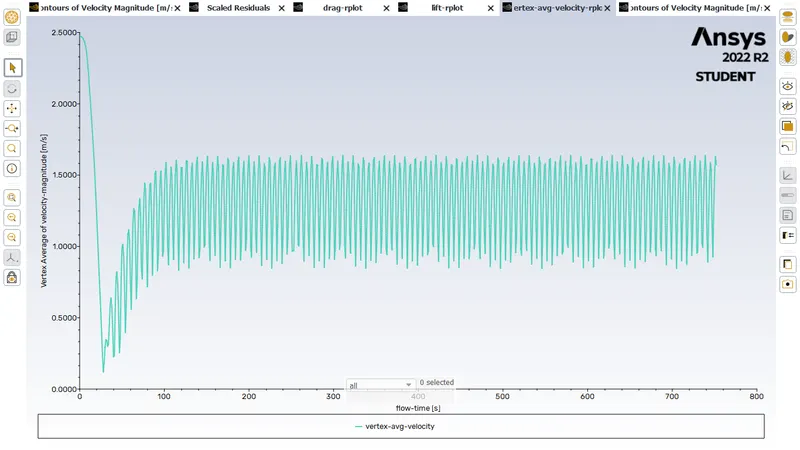
Please refer the below photo for the Vertex-Avg-Velocity plot obtained.

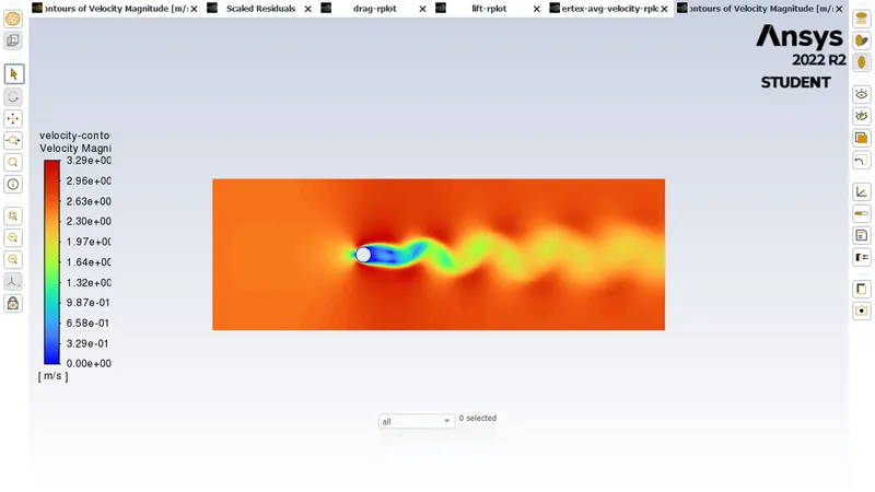
Please refer the below photo for the Velocity contour plot obtained.

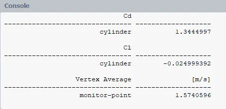
Please refer the below photo for the values obtained for the above plots.

Please refer the below photo for the Magnitude VS Strouhal number obtained.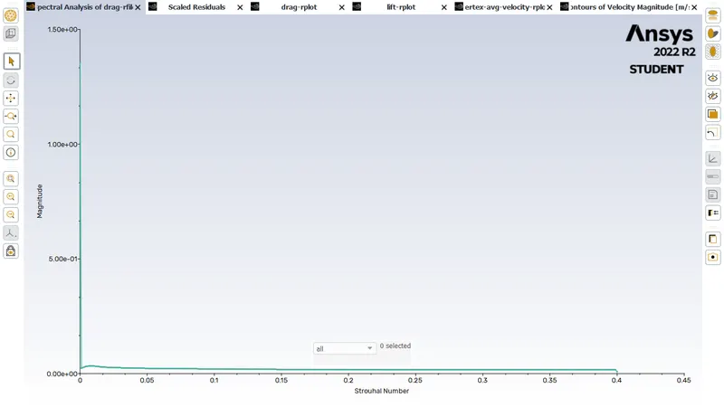

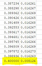
Strouhal number obtained is 0.008126 as highlighted in the above photo from the graph values.

PART II RESULTS:

For study flow for the Reynolds number 10.

Please refer the below photo for the Residuals obtained.

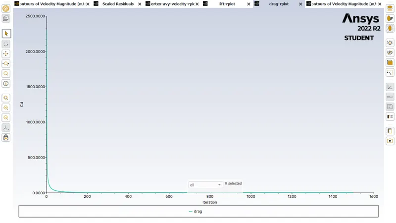
Please refer the below photo for the Drag plot obtained.

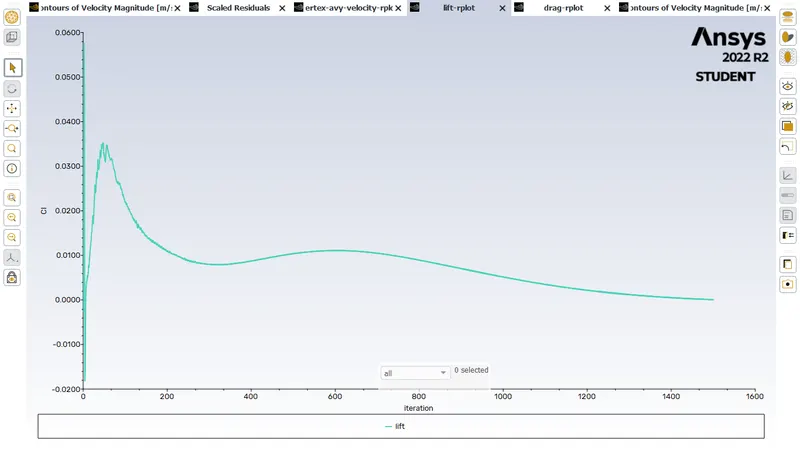
Please refer the below photo for the Lift plot obtained.

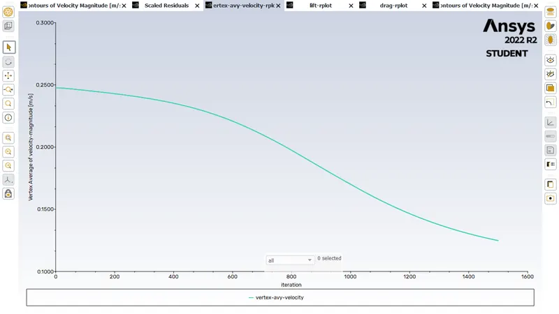
Please refer the below photo for the Vertex-Avg-Velocity plot obtained.

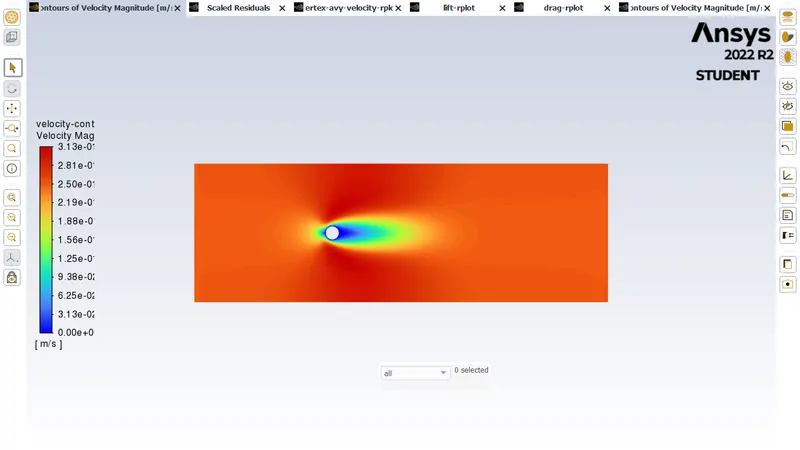
Please refer the below photo for the Velocity contour plot obtained.

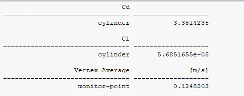
Please refer the below photo for the values obtained for the above plots.

Please refer the below photo for the Magnitude VS Strouhal number obtained.

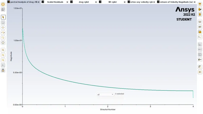
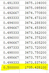
Strouhal number obtained is 1735.4281 as highlighted in the above photo from the graph values.

For study flow for the Reynolds number 1000.

Please refer the below photo for the Residuals obtained.

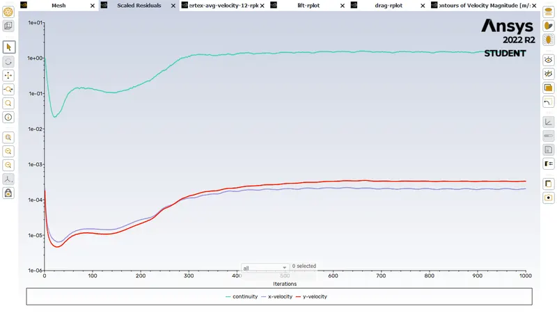
Please refer the below photo for the Drag plot obtained.

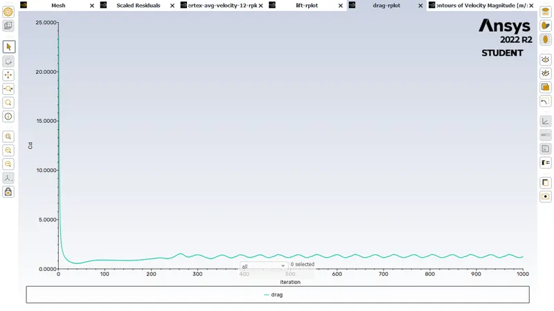
Please refer the below photo for the Lift plot obtained.

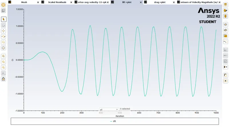
Please refer the below photo for the Vertex-Avg-Velocity plot obtained.

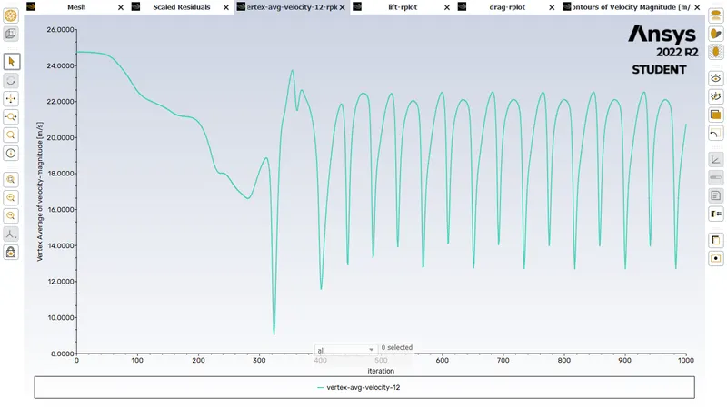
Please refer the below photo for the Velocity contour plot obtained.

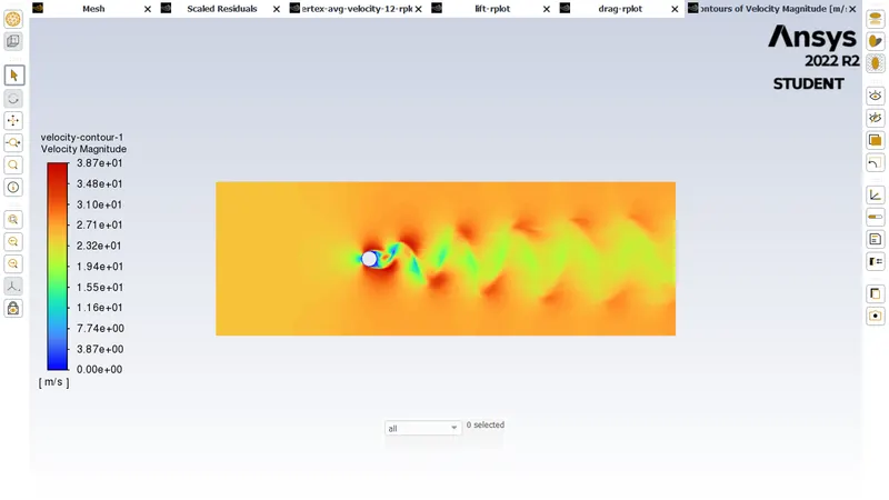
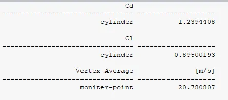
Please refer the below photo for the values obtained for the above plots.

Please refer the below photo for the Magnitude VS Strouhal number obtained.

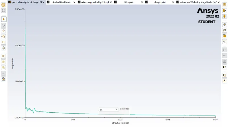
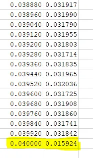
Strouhal number obtained is 0.015924 as highlighted in the above photo from the graph values.

For study flow for the Reynolds number 10000.

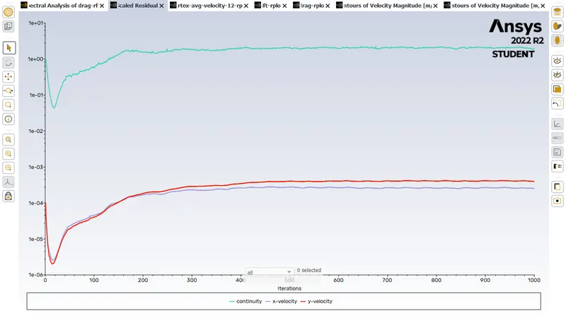
Please refer the below photo for the Residuals obtained.

Please refer the below photo for the Drag plot obtained.

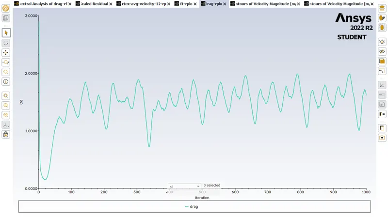
Please refer the below photo for the Lift plot obtained.

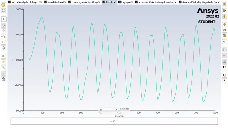
Please refer the below photo for the Vertex-Avg-Velocity plot obtained.

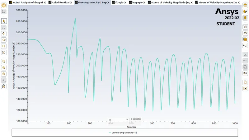
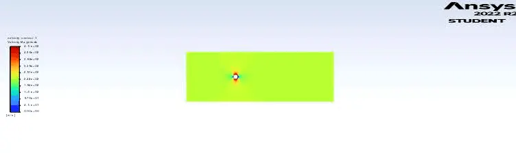
Please refer the below photo for the Velocity contour plot obtained.

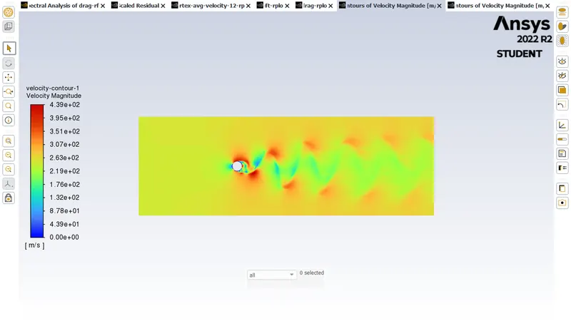
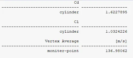
Please refer the below photo for the values obtained for the above plots.

Please refer the below photo for the Magnitude VS Strouhal number obtained.

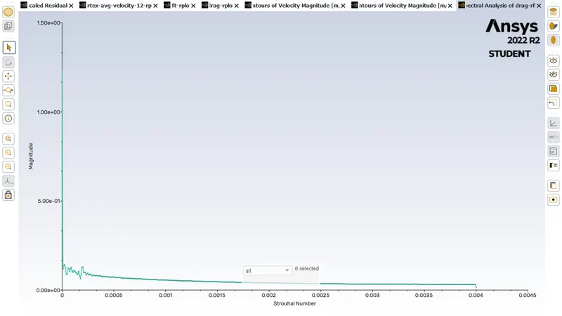
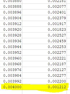
Strouhal number obtained is 0.001212 as highlighted in the above photo from the graph values.

For study flow for the Reynolds number 100000.

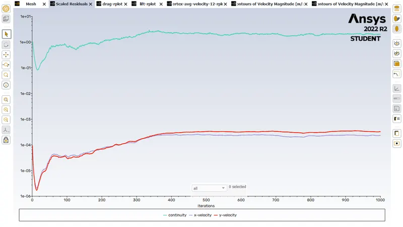
Please refer the below photo for the Residuals obtained.

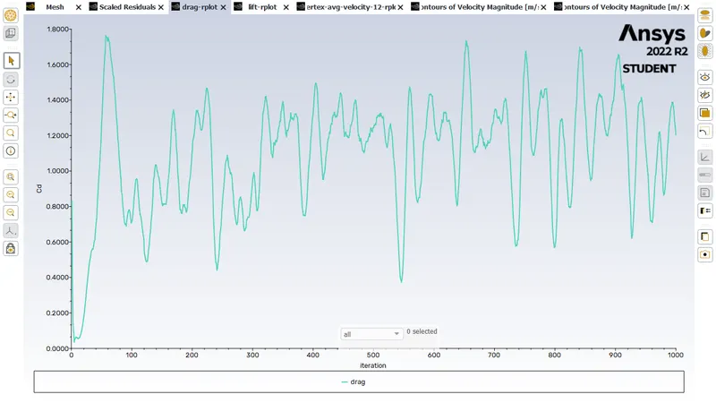
Please refer the below photo for the Drag plot obtained.

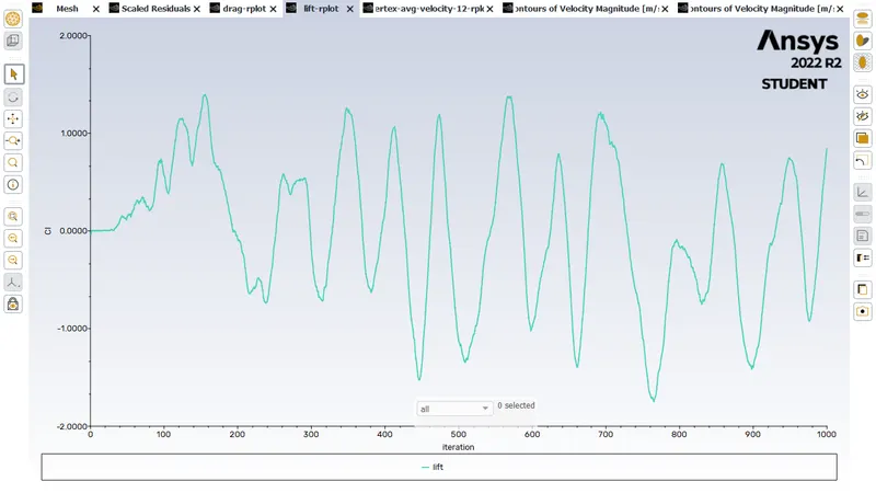
Please refer the below photo for the Lift plot obtained.

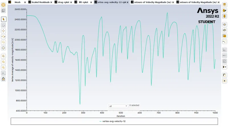
Please refer the below photo for the Vertex-Avg-Velocity plot obtained.

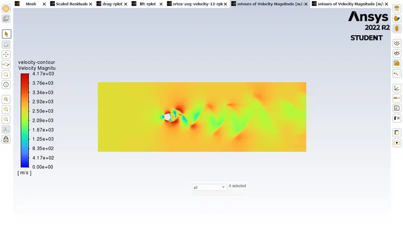
Please refer the below photo for the Velocity contour plot obtained.

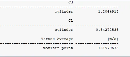
Please refer the below photo for the values obtained for the above plots.

Please refer the below photo for the Magnitude VS Strouhal number obtained.

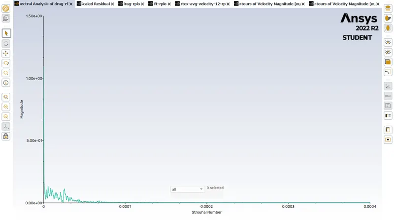
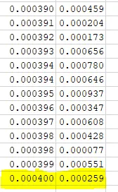
Strouhal number obtained is 0.000259 as highlighted in the above photo from the graph values.

Numarical results obtained as in the below table

Reynolds number	Type of flow	Inlet velocity in m/s	Vertex average velocity in m/s	Drag coefficient Cd	Lift coefficient Cl	Strouhal number
10	Study	0.25	0.1248	3.3814	0.0000568	1735.428
100	Study	2.5	1.8151	1.3538	0.002152	0.16126
100	Unstudy	2.5	1.5740	1.3444	-0.02499	0.008126
1000	Study	25	20.7808	1.2394	0.8950	0.015924
10000	Study	250	136.9806	1.62278	1.03242	0.001212
100000	Study	2500	1619.9573	1.2044	0.84272	0.000259

Validation for the Reynolds number 100 in study state from the standard literature refered.

From the research paper the values obtained is in the below table highlighted.

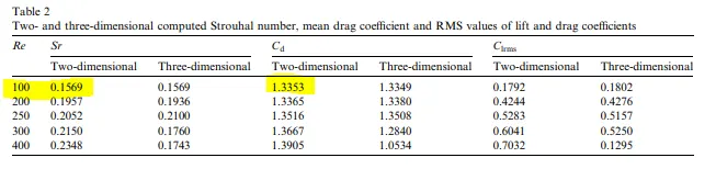
Drag coefficient of standard literature is 1.3353 aobtained values is 1.3538

%error obtained is (1.3538-1.3353)/1.3353*100=1.38%

Strouhal number of standard literature is 0.1569 aobtained values is 0.16126

%error obtained is (0.16126-0.1569)/0.1569*100=2.77%

For Reynolds number 100 study state and unstudy state the Strouhal number around 2.77% and 94% error respectively so prefer to study state only.

CONCLUSION:

Please refer the below graph for the relation between Reynolds number and Vertex average velocity

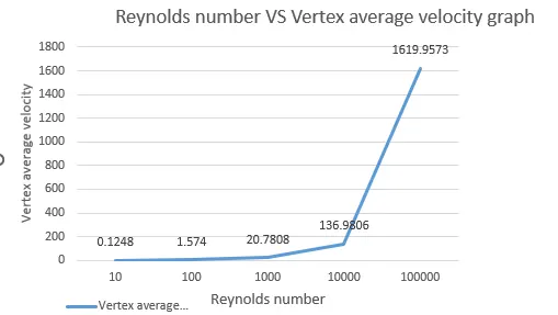
From the above graph we can conclude that as the reynolds number increases the Vertex average velocity also increases.

Please refer the below graph for the relation between Reynolds number and Strouhal number

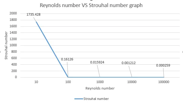
From the above graph we can conclude that as the reynolds number increases the Strouhal number decreases.

Please refer the below graph for the relation between Reynolds number and Drag and lift coefficient (Cd Cl)

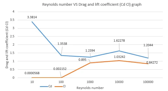
From the above graph we can conclude that as the reynolds number increases the Drag coefficient (Cd) decreases and Lift coefficient (Cl) increases.

I have refer this Research Paper which is linked here https://drive.google.com/file/d/1bKprjY54fSDCIHSdK8YvK4Xyuh3Q0KOo/view?usp=sharing