Week 4 - CHT Analysis on Exhaust port
Aim: To perform the steady-state conjugate heat transfer simulation on the exhaust port with the air velocity of 5m/s at four inlet and one outlet.
Objective:
- Give a brief description of why and where a CHT analysis is used.
- Maintain the y+ value according to the turbulence model and justify the results.
- Calculate the wall/surface heat transfer coefficient on the internal solid surface & show the velocity & temperature contours in appropriate areas.
- Verify if the HTC predictions from the simulations are right, On what factors does the accuracy of the prediction depend on?
Theory:
Heat:
Heat is a form of energy that exist due to the temperature difference. Heat transfer can be defined as the transmission of energy from one region to another region as a result of temperature difference.
There are three basic modes of heat transfer.
- Conduction: This is the mode of heat transfer in which energy exchange takes place due to temperature difference by kinetic motion, direct impact of molecules example metals
- Convection: This is the mode of heat transfer in which energy exchange takes place due to the temperature difference by the macroscopic motion of fluid particles.
- Radiation: This is the mode of heat transfer in which the energy exchange takes place without the aid of any intervening medium.
Fourier Law of heat transfer:
The law of heat conduction based on experimental observation is known as the Fourier’s Law which state that “ The rate of heat flow by conduction in a given direction is proportional to the area normal the direction of the heat flow and also temperature gradient in that direction”.
It is given by the below formula
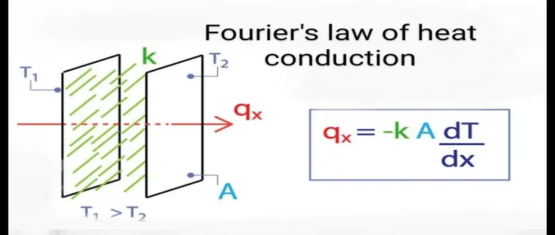
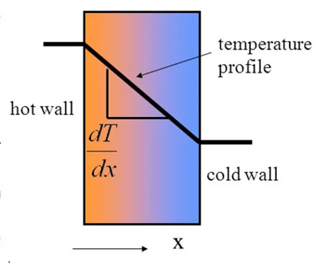
Where qx is the rate of heat flow in Watts or J/s
A is the areas normal to the direction of heat transfer in m2
dT/dx is the Temperature gradient in °K/m
-ve sign indicated that heat flows from higher temperature to lower temperature.
k, is called thermal conductivity of the material, it is the property of the material which varies with temperature.
Thermal conductivity (k):
Thermal conductivity of a metal can be define as the rate of heat transfer through a unit thickness of the material per unit area per unit temperature difference.
The unit of Thermal conductivity is W/m-°K
A higher the value of thermal conductivity indicates that the material is good heat conductor and low value indicates poor heat conductor or insulator.
Newtons Cooling Law:
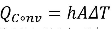
It states that convective heat transfer is proportional to the difference in temperature between an object and its surrounding area.
It is given by the below formula
 ------------1
Where QConv is the Convective heat transfer per unit time
h is the heat transfer coefficient W/m2 °K
A is the Normal surface area in m2.
^T is the temperature difference in °K
Convective is a mode of energy transfer that involves the combine effect of conduction and fluid motion between the solid surface and an adjacent moving liquid or gas.
Faster the fluid flow higher the convective heat transfer.
Thermal diffusivity:
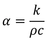
Thermal diffusivity is the measure of the ratio of heat conducted to the heat stored and consequently can be used qualitatively to predict how fast the temperature of the body changes. A material.
It is given by the below equation:
 ------------------2
Where α is the thermal diffusivity in m2/s
k is Thermal conductivity in W/m-°K
𝜌 is the density in kg/m3
C is the Specific heat capacity in kJ/kg °K
The larger values of α for higher value of k and lower value of 𝜌c leads to the faster heat dissipation in the material.
Higher the value of k will result in the faster energy transfer though the material
Lower the value of c means lesser amount of heat moving through the material will be used for raising the temperature and more of it will be available for transferring.
Specific heat capacity (c) :
Specific heat capacity is defined as the amount of energy require to rise the temperature by 1 °C per unit kg of the substance.
Its SI unit is KJ/kg °K
There are 2 types of convection heat transfer.
- Forced convection
- Free or Natural convection
1) Forced convection
When a fluid is forced to flow over the surface by an internal source such as fans, by stirring, and pumps, creating an artificially induced convection current
2) Free or Natural convection
The mechanism of heat transfer in natural convection involves the motion of fluid particles past a solid boundary which is a result of the density differences resulting from the energy exchange. As a result, the heat transfer coefficients will vary with the geometry
“h” heat transfer coefficient is not a property it’s a experimentally determined parameter like temperature, surface geometry and velocity of the fluid.
Reynolds number:
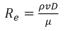
Reynolds number is a dimensionless quantity that is used to determine the type of flow pattern as laminar or turbulent while flowing through a pipe. Reynolds number is defined by the ratio of inertial forces to that of viscous forces.
It is given by
 ----------------3
Re is the Reynolds number
ρ is the density of the fluid (kg/m³)
V is the velocity of flow (m/s)
D is the pipe diameter (m)
μ is the viscosity of the fluid (kg/m-s)
Nusselt number:
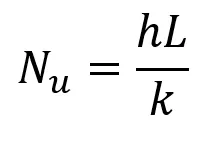
It is the ratio of convective heat transfer to the conductive heat transfer within the fluid range.
It is given by the equation
 ---------------4
Nu is the dimensionless Nusselt number
h is the heat transfer coefficient W/m2 °K
L is the length or diameter of the geometry in m
k is Thermal conductivity in W/m-°K
Nusselt number denotes the increase in the heat transfer through a fluid layer caused by the convection, relative to conduction.
When a fluid is motionless (no bulk motion) conduction will be the dominating mode of heat transfer
When there is a bulk motion, the convection will be higher.
Prandtl number:
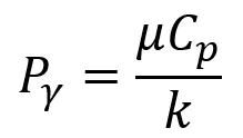
It is the ratio of momentum diffusivity to the thermal diffusivity.
It compares the velocity boundary layer thickness to the thermal boundary layer thickness (which boundary layer is thicker)
This number represents the relative importance of momentum and energy transfer by diffusion process
For gas, Prandtl number is 1 and therefore the transfer of momentum energy by diffusion is comparable.
For oils, Prandtl number is greater than 1 hence the momentum diffusion is much greater than energy diffusion.
For water Prandtl number is in the order of 10.
Prandtl number is 0.01 for liquid metals and 10^5 for heavy oils
It is given by the equation
 -------------5
Whare Pr is the Dimensionless Prandtl number
μ is the viscosity of the fluid in kg/m-s
Cp is the specific heat at constant pressure in J/kg °K
k is the Thermal conductivity in W/m-°K
Dittus–Boelter equation:
The Dittus–Boelter equation (for turbulent flow) as introduced by W.H. McAdams is an explicit function for calculating the Nusselt number. It is easy to solve but is less accurate when there is a large temperature difference across the fluid. It is tailored to smooth tubes, so use for rough tubes (most commercial applications) is cautioned. The Dittus–Boelter equation is:
 --------------6
where:
Nu is the dimensionless Nusselt number
Pr is the Dimensionless Prandtl number
Re is the Reynolds number
n=0.4 for heating of fluids
n=0.3 for cooling of fluids
Calculation of heat transfer coefficient(h)
Following data is given:
ρ, density of the fluid 1.225 kg/m³
V, velocity of flow 5 m/s
D or L, pipe diameter 0.166 m
μ, viscosity of the fluid 1.7894x10^-5 kg/m-s
Cp, specific heat at constant pressure 1006.43 J/kg °K
k, Thermal conductivity 0.0242 W/m-°K
By applying these input values to Reynolds number equation 3 we get
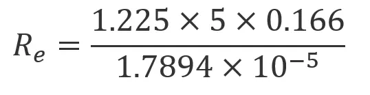
Reynolds number obtained is 56,820.722
By applying above input values to Prandtl number equation 5 we get
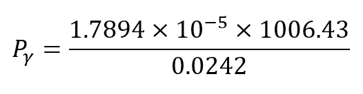
Prandtl number obtained is 0.74417
From these Reynolds number and Prandtl number find the value of Nusselt number by using Dittus–Boelter equation 6 we got

Nusselt number obtained is 133.916
From the below equation put all the values except h which is is the heat transfer coefficient to be calculated.
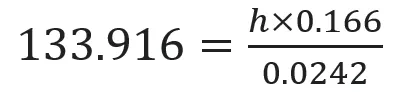
By solving the above equation we obtain heat transfer coefficient h as 19.5226 W/m2-°K
Theoritical Y+ calculation:
We have calculated the Reynolds number above and is 56,820.722
Skin-Friction Drag and Skin-Friction Coefficient (Cf):
Skin friction drag is a type of aerodynamic or hydro dynamic, which is resistant force exerted on an object moving in a fluid. Skin friction drag is caused by the viscosity of fluids and is developed from laminar drag to turbulent drag as a fluid moves on the surface of an object. Skin friction drag is generally expressed in terms of the Reynolds number. The skin friction coefficient is a dimensionless skin shear stress which is nondimensionalized by the dynamic pressure of the free stream. The skin friction coefficient is defined at any point of a surface that is subjected to the free stream. The skin friction coefficient is a strong function of the Reynolds number, as Reynolds number increases Skin-Friction Coefficient decreases.
Theoritically it is given by
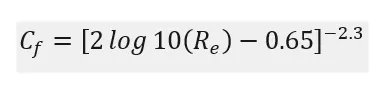

Finaly we obtain Skin-Friction Coefficient as 0.006622
Wall Shear Stress (τw):
Wall shear stress expresses the retarding force (per unit area) from a wall in the layers of a fluid flowing next to the wall. It is given by the below equation
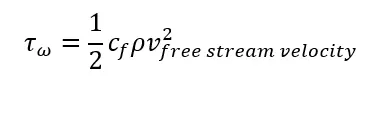
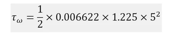
Finaly we obtain Wall Shear Stress (τw) as 0.1014 Pa
Friction Velocity (U*):
Shear velocity, also called friction velocity, is a form by which a shear stress may be re-written in units of velocity. It is useful as a method in fluid mechanics to compare true velocities, such as the velocity of a flow in a stream, to a velocity that relates shear between layers of flow. It is given by the equation
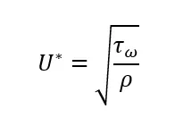
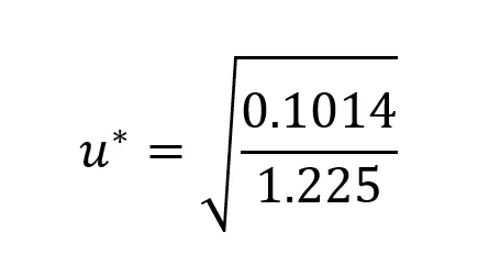
Finaly we obtain Friction Velocity (U*) as 0.287707 m/s
Wall Distance (y):
Wall distance (y) is the vertical distance measured from the wall. It is given by the equation
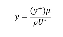
Here we have to maintain the Y+ value wit respect to the turbulance model
For RNS model of K- epsalon, the range of y+ is 30-300
For K-omega-SST model the range of y+ is 0-5.
In this case we are using K-omega-SST so taken y+ as 1
By putting the respective values in the above equation
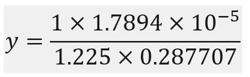
Finaly we obtain Wall distance (y) as 0.0000507716 m
For turbulance boundry layer thickness (𝞭99) from Cengel and Cimbala emperical formula is
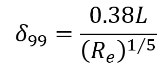
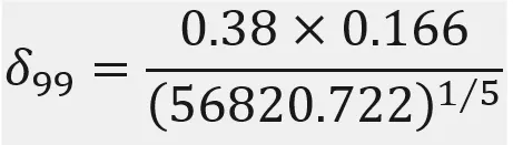
Turbulance boundry layer thickness (𝞭99) obtained is 0.00706301 m
For the growth rate of 1.2 the number of Prism layer is caluculated by the geometric progression formula and is given by
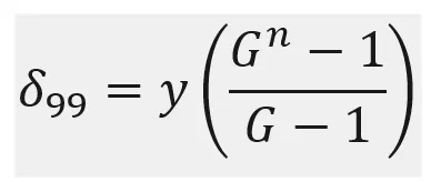

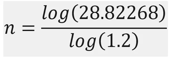
Finaly we obtain the number of Prism layer as 18.4353 we can take it as 19 prism layer.
Theory on conjugate heat transfer (CHT) :
In certain critical applications where, working temperature is very high, it is necessary to calculate the temperature distribution in the solid to ensure that it should not cross the metallurgical limit. The Selection of the material and wall thickness is largely dependent on the wall temperature distribution in the solid. Hence, it is necessary to solve the energy equation of the solid along with the fluid flow equations, commonly known as conjugate heat transfer problem. This type of problem differs from commonly encountered heat conduction problems, as the temperature of the fluid which is used to cool (or heat) the solid is known a priori. Instead, the fluid temperature is calculated at the same time as the solid temperature. In most of the earlier works, the temperature distribution in the boundary layer of the main stream is determined under a prescribed condition at the surface and then the heat transfer coefficient is calculated. Next the heat transfer process in the solid is calculated. Thus, the complexity of the heat transfer processes between the fluid and the main stream is described by a pre-determined heat transfer coefficient which shows heat transfer process is independent of the solid properties. Contrary, the recent works of the convective heat transfer problems with conjugate heat transfer seems to be more physical compared to the earlier works as the calculations for the fluid and the solid are done simultaneously.
The works reported in the field of conjugate heat transfer are mostly analytical. Few experimental studies are made for laminar and turbulent flow. Numerical studies are relatively scarce. The geometries taken into consideration are flow over flat plate, flow between heated parallel plates or rectangular ducts, surface mounted heat blocks in forced or natural flow, finned-tube in cross flow, circular cylinders in uniform flow etc.
CHT represents a class of multi-physics problems where fluid flow affects the thermal behaviour of structure, which in turn affects the fluid flow. For conjugate heat transfer analyses, the solid material conduction and the fluid convection are analysed simultaneously. The conductive heat transfer in a solid region is coupled to the convective heat transfer in a neighbouring fluid flow.
The computational domain of a CHT problem consists of the fluid domain and solid domain. In fluid domain, the three-dimensional Navier-Stokes equations are solved for velocity components, pressure, density, temperature etc. In the CHT solid, diffusion is the only transport process, and only the energy equation is solved for temperature. The fluid energy and the solid energy equations are coupled for the identical conditions of temperature and heat flux at the solid-fluid interface. The governing equations in fluid and solid are solved using the 3-D Navier-Stokes Code-CFX TASC Flow which is an integrated software system capable of solving diverse and complex multidimensional fluid flow problems. The code is fully implicit, finite volume method with finite element-based discretization of geometry. It utilizes numerical upward schemes to ensure global convergence of mass, momentum and energy. It implements a general non-orthogonal, structured, body fitted grids. In the present study, the discretization of the convective terms is done by first order upwind difference scheme. The turbulence model used was k – omega SST model with wall functions.
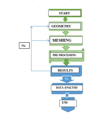
Please refer the below chrt for the CFD work flow analysis of the conjugate heat transfer simulation on the exhaust port.
Geometry set-up:
We have to follow the following steps in the Geometry set-up.
- Import the geometry.
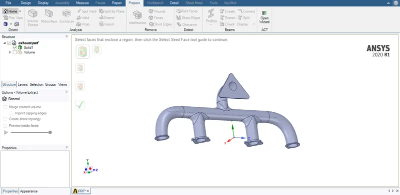
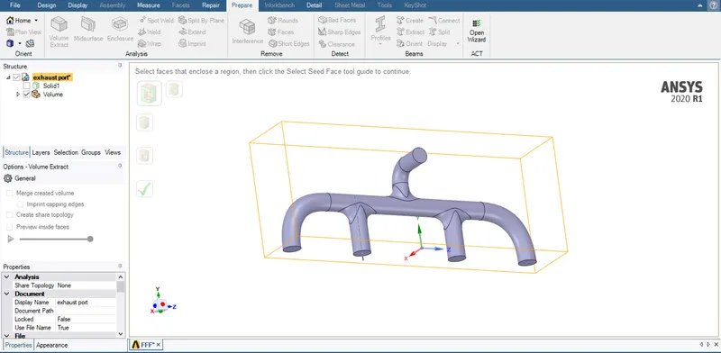
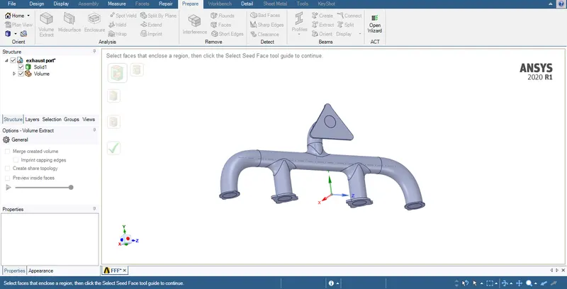
- Extraction of fluid volume by using volume extract tool.
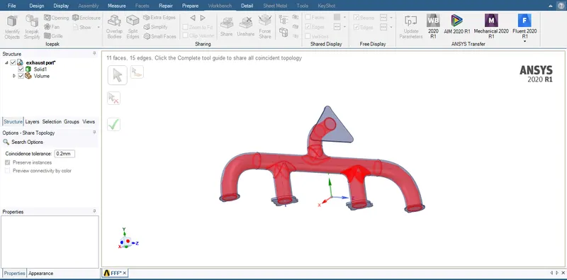
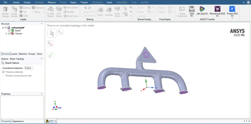
- Sharing the topology by using share tool which is available in the workbench.
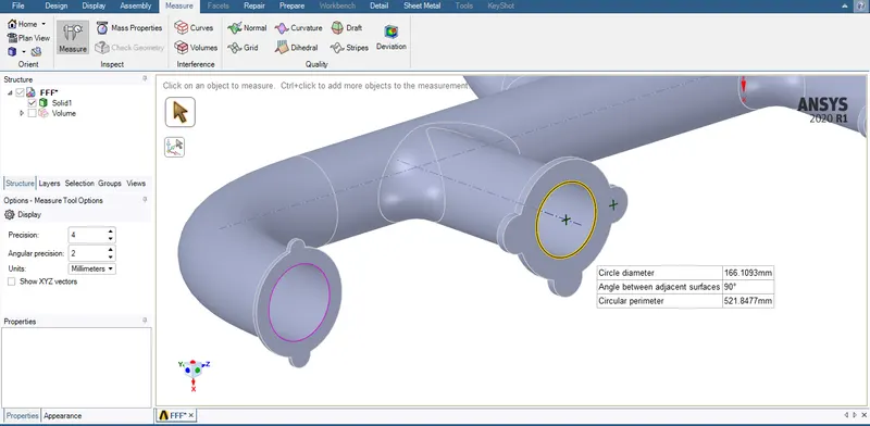
Please refer the below photo for the imported geometry and diameter of the inlet pipe which is 166 mm or 0.166 m.
Please refer the below photo for the Extraction of fluid volume by using volume extract tool.
Please refer the below photo for before and after Sharing the topology applied respectively.
Meshing Set-up:
Following steps were followed in the Meshing Set-up.
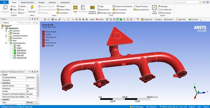
- Nomenclature of exhaust port as inlet, outlet, solid domine, fluid domine, fluid wall and external wall.
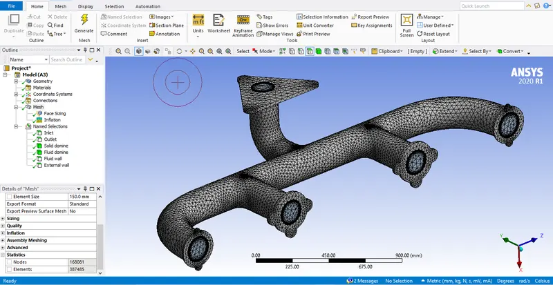
- Meshing the solid domine.
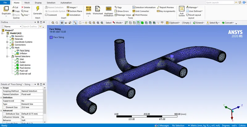
- Body sizing the fluid domine.
- Creating an inflation layer.
- Performence mesh independent study for 5 cases.
Please refer the below photo for Nomenclature of exhaust port.
Please refer the below photo for Meshing the solid domine, element size given is 150 mm.
Please refer the below photo for Body sizing the fluid dominel, element size given is 25 mm.
Inflation layer calculation online Y+ calculator VOLUPE software as shown below.
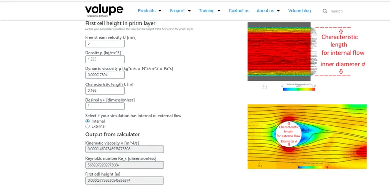
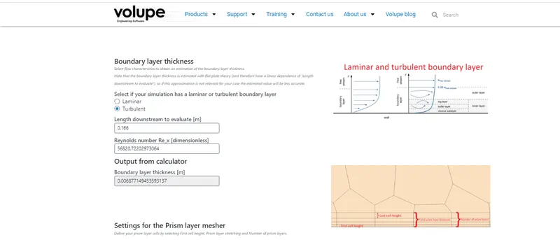
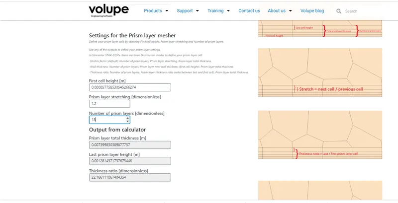
First cell height is 0.000057758 m and growth rate is 1.2 to match the prism layer total thickness boundry layer thickness by adjusting the number of prism layers as 18, but for good volume transition we should increase the number of prism layers as 25.
Please refer the below photo for the Inflation layer obtained.
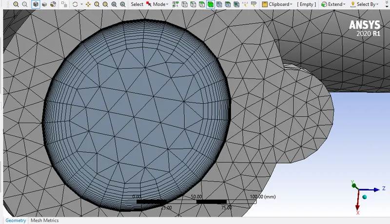
Performence mesh independent study for 5 different cases as in the below table.
| Case | Mesh element size for solid domine in mm | Mesh element size for Fluid domine in mm |
| 1 | 150 | 25 |
| 2 | 130 | 20 |
| 3 | 110 | 15 |
| 4 | 90 | 10 |
| 5 | 80 | 8 |
Case 1:
Please refer the below photo for the number of nodes and elements obtained in the case 1 is 168081 and 387485 respectively.
Please refer the below photo for the mesh element quality obtained, average value is 0.2704
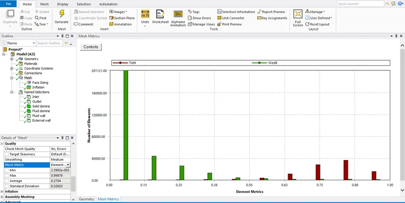
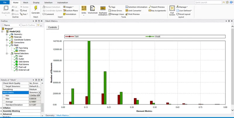
Please refer the below photo for the mesh Skewness obtained, average value is 0.19897
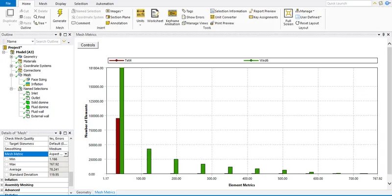
Please refer the below photo for the mesh Aspect ratio obtained , average value is 78.24
Fluent set up:
Please refer the below table for the fluent set-up inputs
| Fluent setup | |
| Solver type | Pressure base |
| Solver time | Steady state |
| Energy | on |
| Turbulance model | k-omega-SST |
| Material fluid | Air for inlet fluid domine, Al for outer body external domine |
| Inlet | Velocity inlet (5 m/s), Temperature |
| Outlet | Pressure outlet |
| External wall, wall-convection | 20 W/m2 °K |
| Internal solid surface | Wall boundary condition |
| Method | Coupled |
Please refer the below photo for the solver type, solver time and energy on applied.

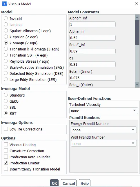
Please refer the below photo for the turbulance model applied.
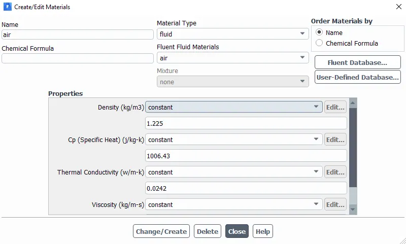
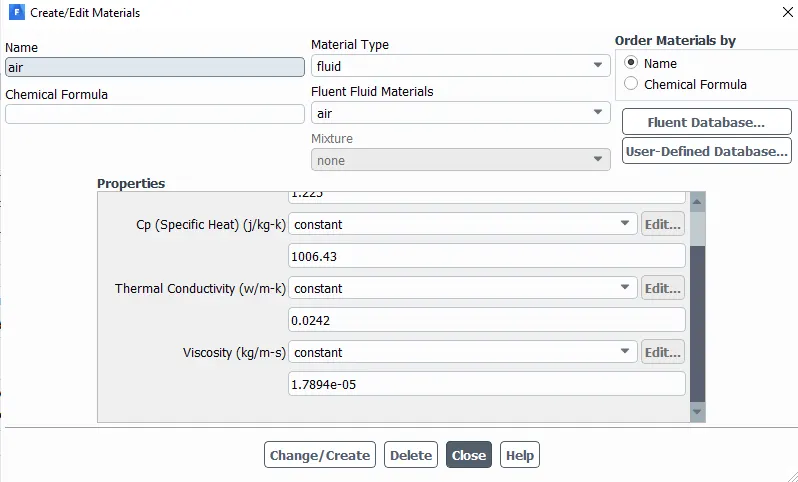
Please refer the below photo for the air material applied and its property.
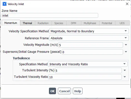
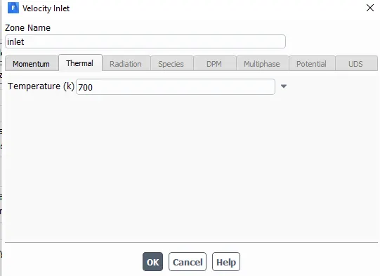
Please refer the below photo for inlet velocity 5 m/s and temperature 700 °K applied.
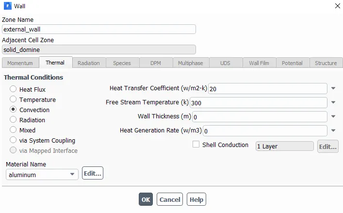
Please refer the below photo for External wall property applied.
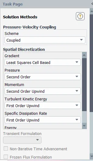
Please refer the below photo for Solution method applied.
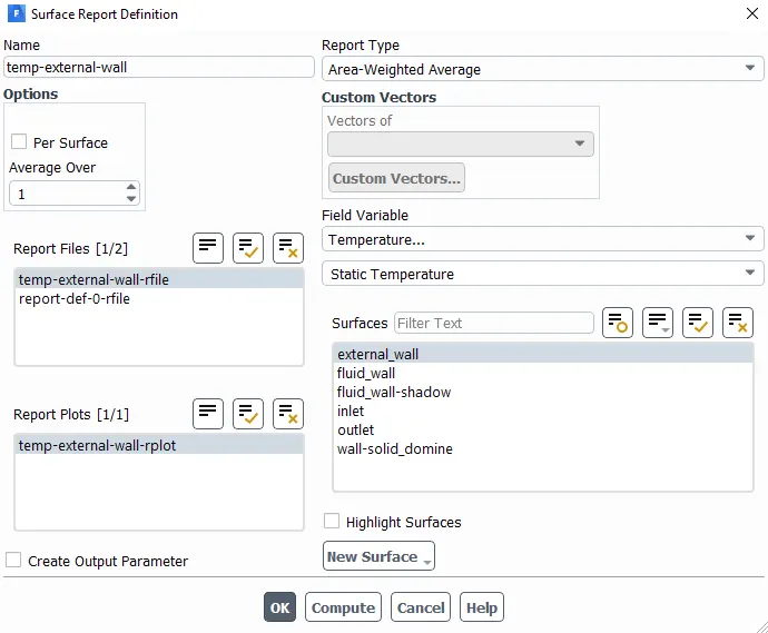
Please refer the below photo for report defination applied for temperature and heat transfer coefficient respectively.

Please refer the below photo for the hybrid initialization done.

After that run calculation for 300 itiration is done.
These fluent set-up is same for all the cases.
Result:
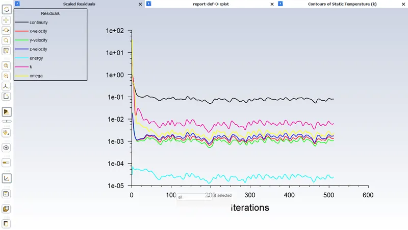
Please refer the below photo for the residuals plots obtained.
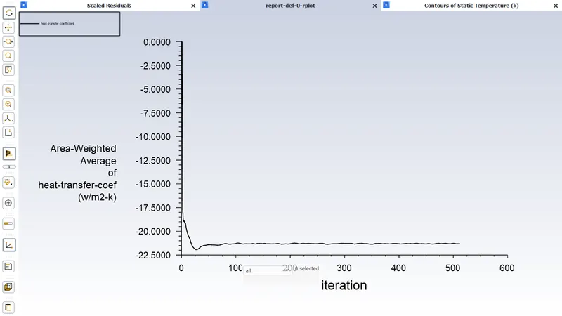
Please refer the below photo for the heat transfer coefficient plot obtained.
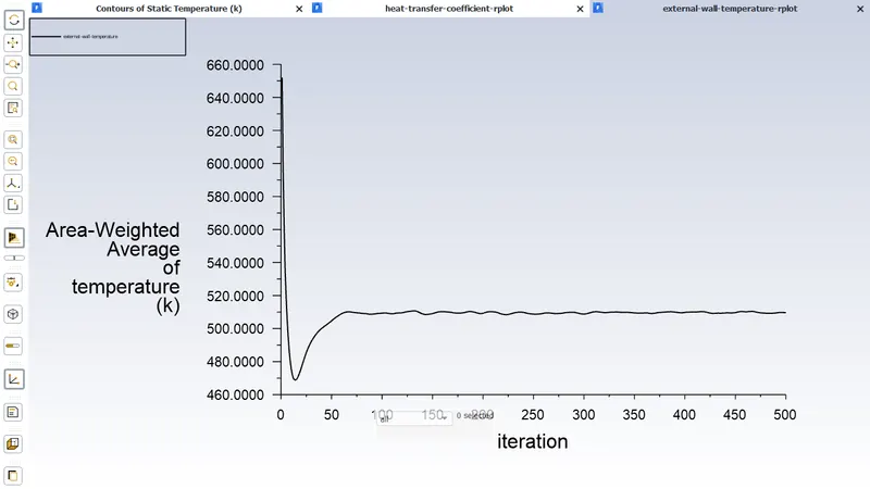
Please refer the below photo for the Temperature plot obtained.
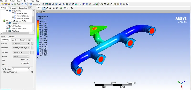
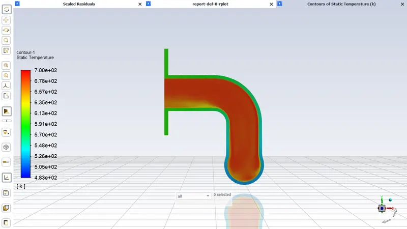
Please refer the below photo for the Temperature Contours obtained and the XY plane view. Due to the sudden bending at the outlet temperature will be decresed after that region outlet
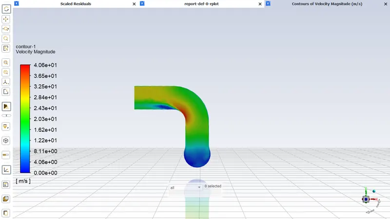
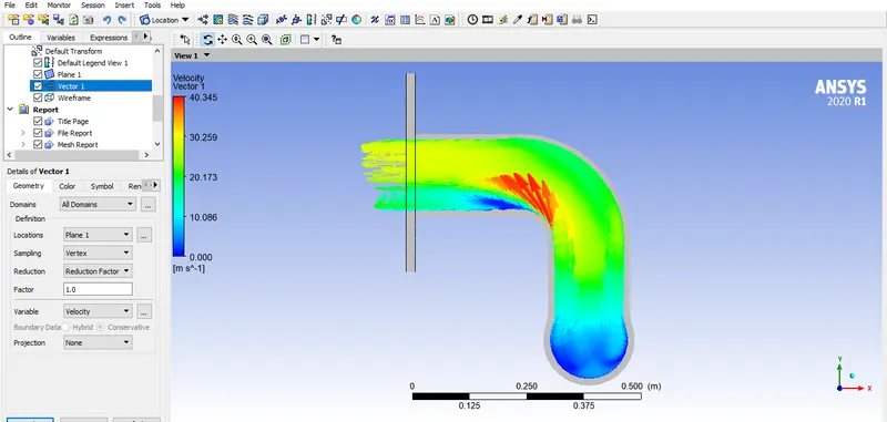
Please refer the below photo for the velocity Contours obtained in XY plane view.Due to the sudden bending at the outlet velocity will be increased littlebit at bend and gradually velocity decreases towards outlet.
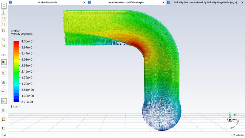
Please refer the below photo for the velocity vector obtained. Due to the sudden bending at the outlet will be increased at bend and graduallythe velocity decreases towards outlet
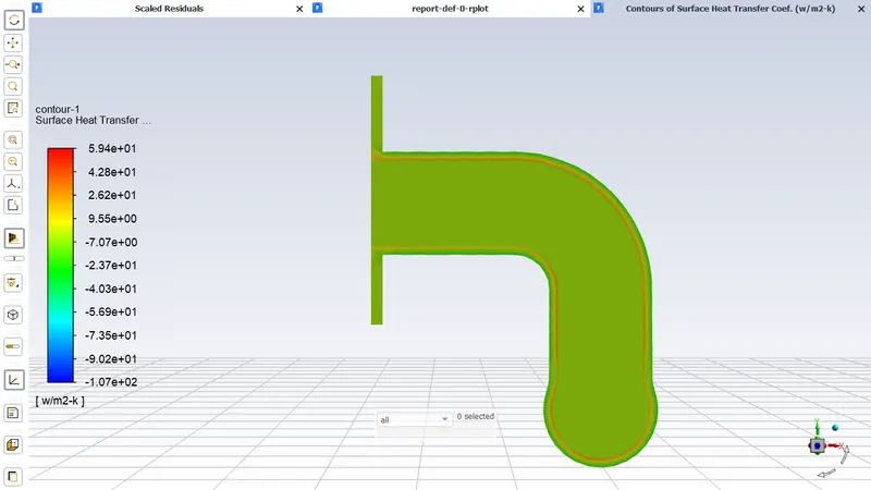
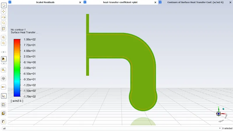
Please refer the below photo for the heat tranfer coefficient Contours obtained. From the below figure it is clear that the heat tranfer coefficient effect will be there at the fluid wall
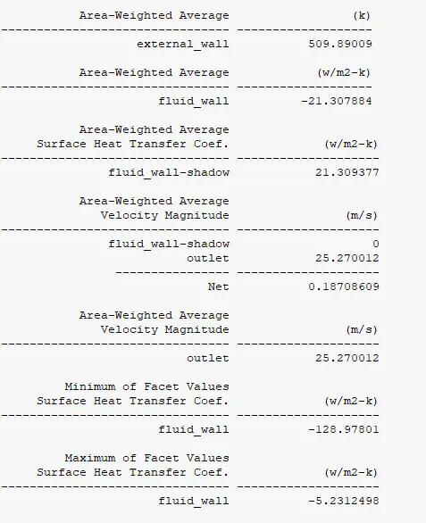
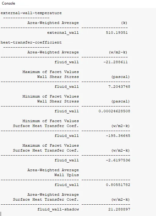
Please refer the below photo for the values obtained. The heat tranfer coefficient obtained is -21.307884 W/m2 °K at the fluid wall and 21.309377 W/m2 °K at the fluid wall shadow, external wall temperature of 509.89009 °K
Case 2:
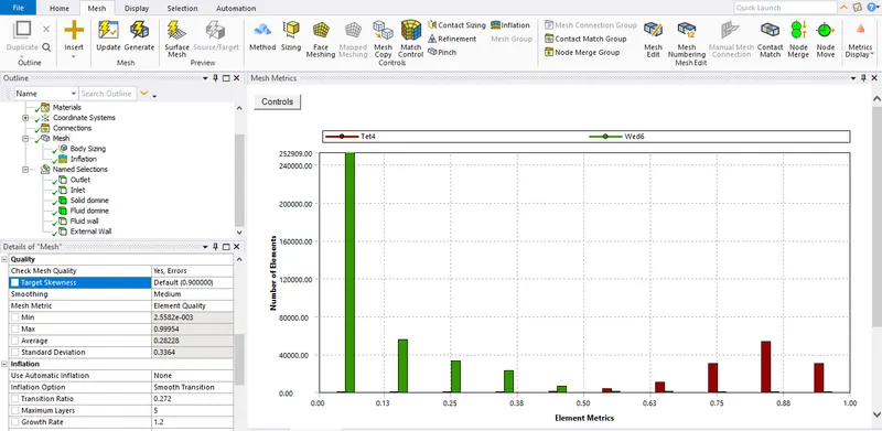
Please refer the below photo for the number of nodes and elements obtained in the case 2 is 213880 and 498773 respectively.
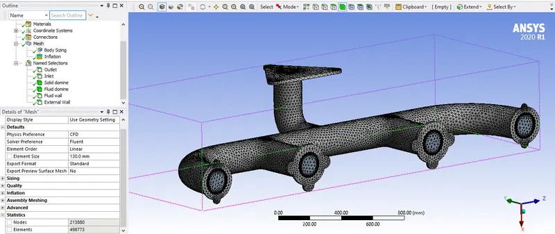
Please refer the below photo for the mesh element quality obtained , average value is 0.28228
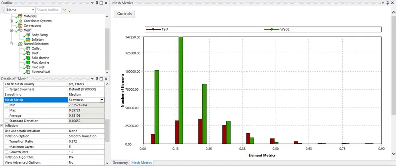
Please refer the below photo for the mesh Skewness obtained , average value is 0.18106
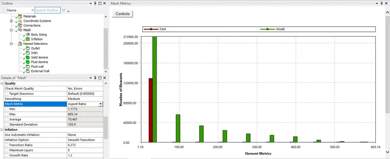
Please refer the below photo for the mesh Aspect ratio obtained , average value is 70.467
Result:
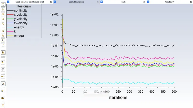
Please refer the below photo for the residuals plots obtained.
Please refer the below photo for the heat transfer coefficient plot obtained.
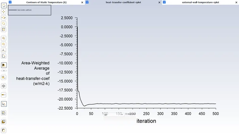
Please refer the below photo for the Temperature plot obtained.
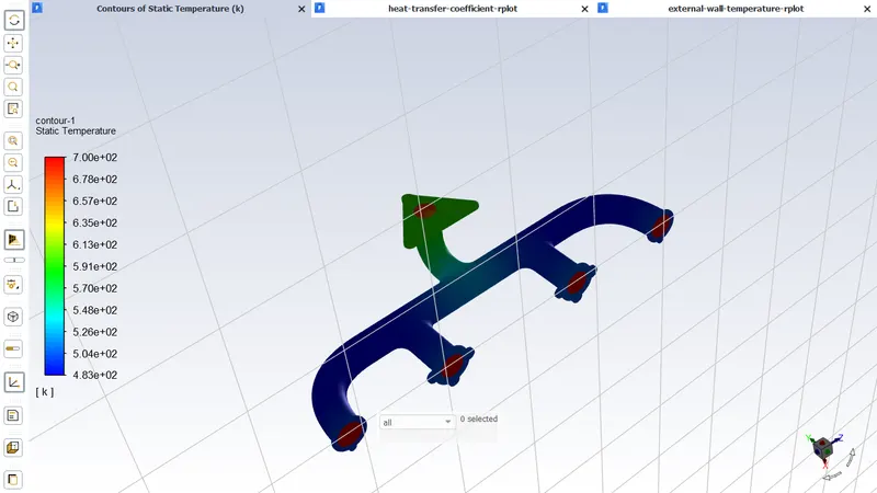
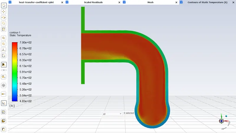
Please refer the below photo for the Temperature Contours obtained and the XY plane view. Due to the sudden bending at the outlet temperature will be decresed after that region outlet
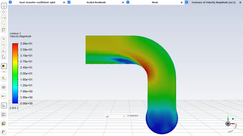
Please refer the below photo for the velocity Contours obtained and the XY plane view. Due to the sudden bending at the outlet velocity will be increased littlebit at bend and gradually velocity decreases towards outlet.
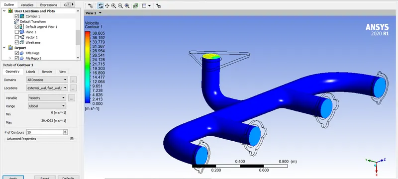
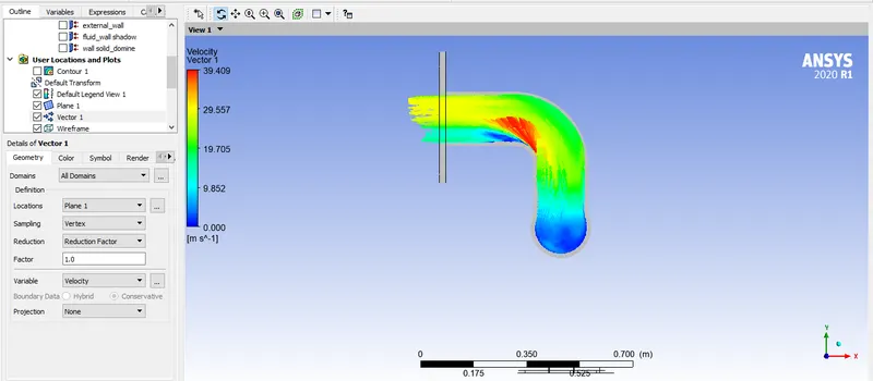
Please refer the below photo for the velocity vector obtained. Due to the sudden bending at the outlet velocity will be increased littlebit at bend and gradually velocity decreases towards outlet.
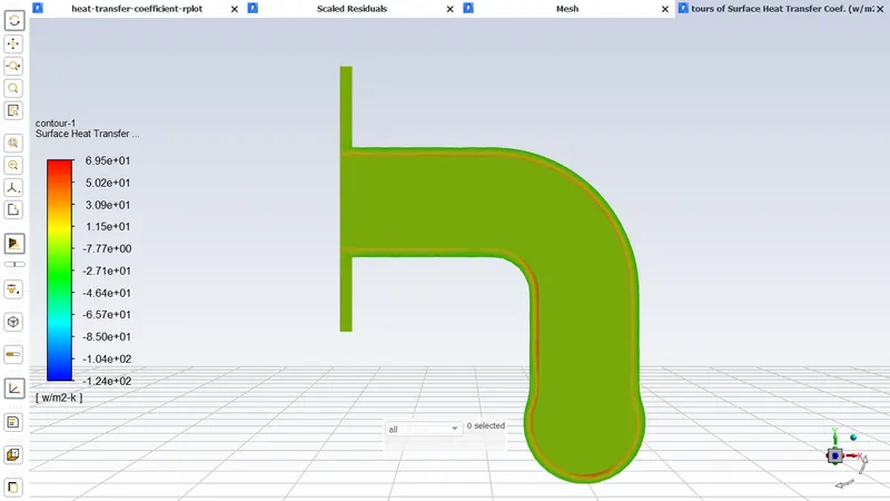
lease refer the below photo for the heat tranfer coefficient Contours obtained. From the below figure it is clear that the heat tranfer coefficient effect will be there at the fluid wall.
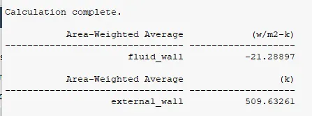
Please refer the below photo for the values obtained. The heat tranfer coefficient obtained is -21.28897 W/m2 °K at the fluid wall and 21.290125 W/m2 °K at the fluid wall shadow, external wall temperature of 509. 63261 °K.
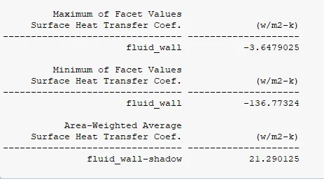
Case 3:
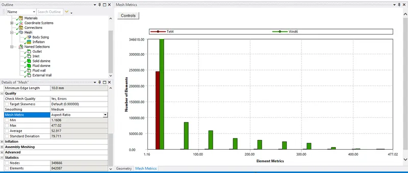
Please refer the below photo for the number of nodes and elements obtained in the case 3 is 349666 and 842087 respectively.
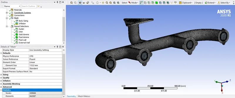
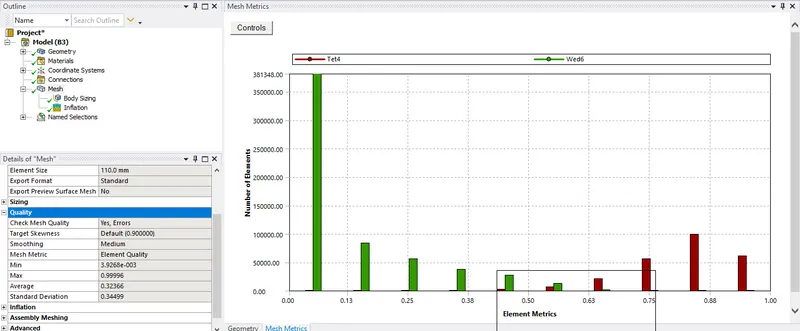
Please refer the below photo for the mesh element quality obtained , average value is 0.32366
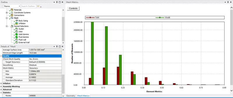
Please refer the below photo for the mesh Skewness obtained , average value is 0.16902
Please refer the below photo for the mesh Aspect ratio obtained , average value is 52.917
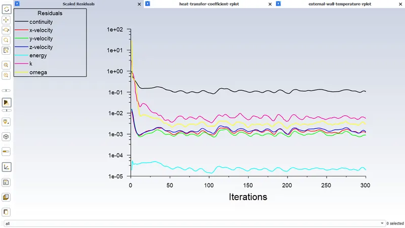
Result:
Please refer the below photo for the residuals plots obtained.
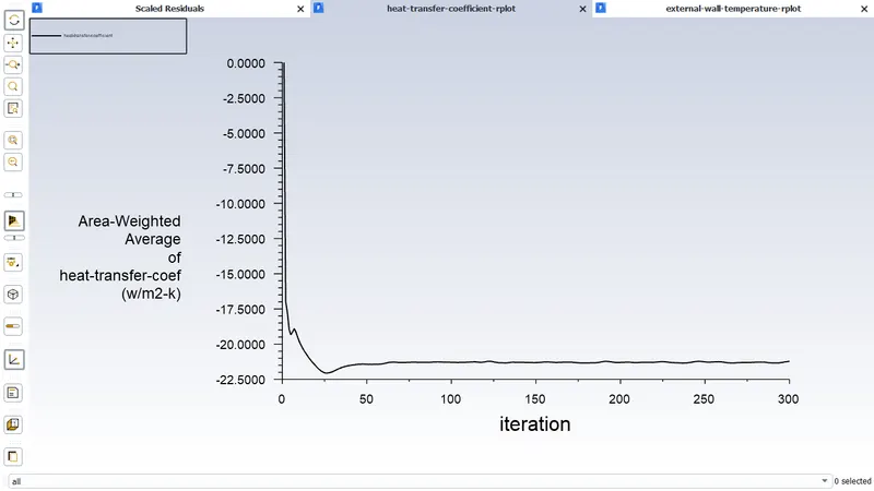
Please refer the below photo for the heat transfer coefficient plot obtained.
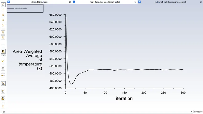
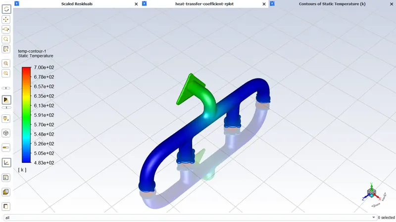
Please refer the below photo for the Temperature plot obtained.
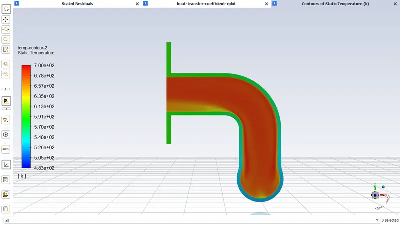
Please refer the below photo for the Temperature Contours obtained and the XY plane view. Due to the sudden bending at the outlet temperature will be decresed after that region outlet
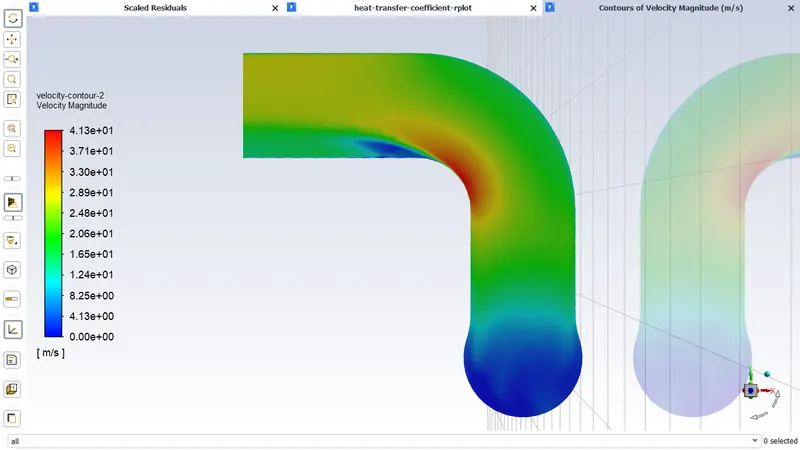
Please refer the below photo for the velocity Contours obtained and the XY plane view. Due to the sudden bending at the outlet velocity will be increased littlebit at bend and gradually velocity decreases towards outlet.
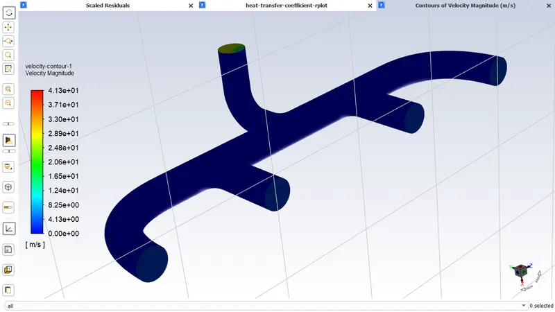
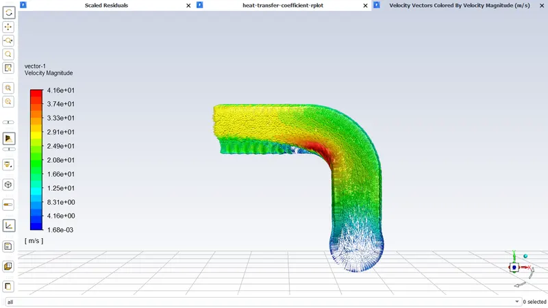
Please refer the below photo for the velocity vector obtained. Due to the sudden bending at the outlet velocity will be increased littlebit at bend and gradually velocity decreases towards outlet.
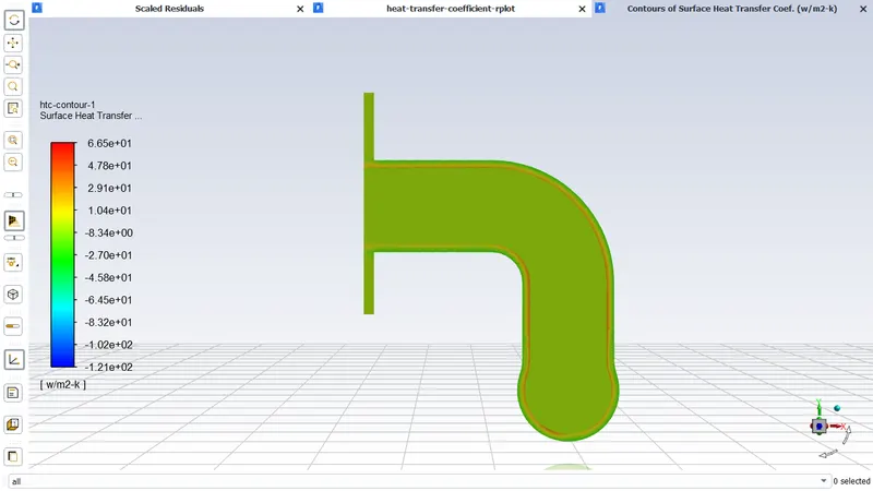
Please refer the below photo for the heat tranfer coefficient obtained. From the below figure it is clear that the heat tranfer coefficient effect will be there at the fluid wall.
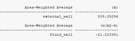
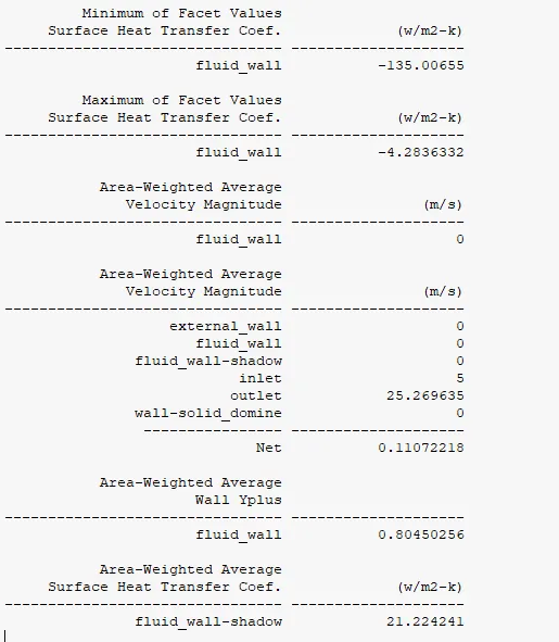
Please refer the below photo for the values obtained. The heat tranfer coefficient obtained is -21.223341 W/m2 °K at the fluid wall and 21.224241 W/m2 °K at the fluid wall shadow, external wall temperature of 509.89296 °K
Case 4:
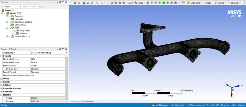
Please refer the below photo for the number of nodes and elements obtained in the case 4 is 831230 and 2167188 respectively.
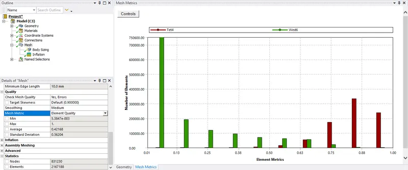
Please refer the below photo for the mesh element quality obtained , average value is 0.42168
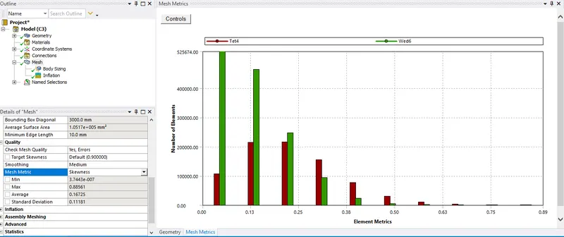
Please refer the below photo for the mesh Skewness obtained , average value is 0.16725
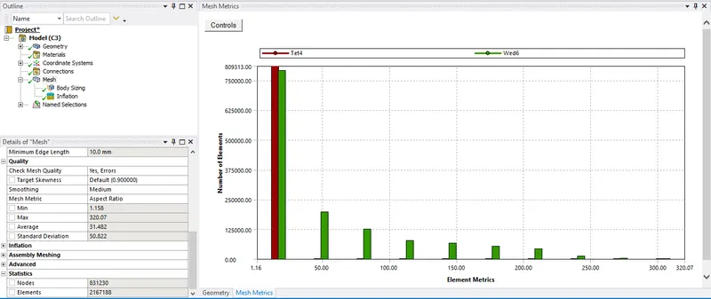
Please refer the below photo for the mesh Aspect ratio obtained , average value is 31.482
Result:
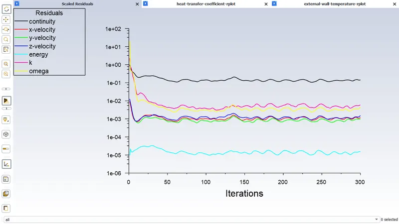
Please refer the below photo for the residuals plots obtained.
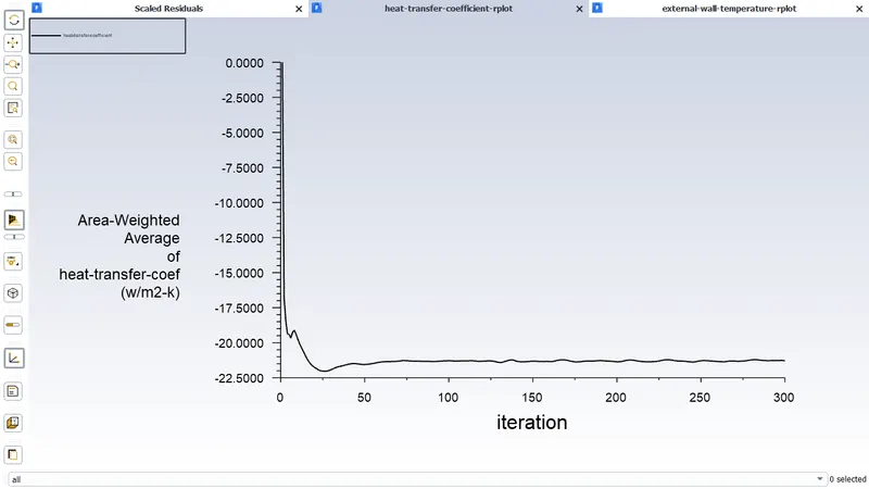
Please refer the below photo for the heat transfer coefficient plot obtained.
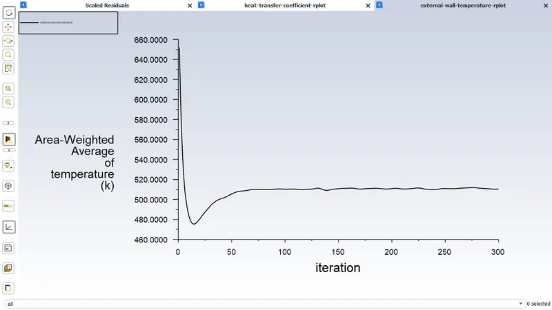
Please refer the below photo for the Temperature plot obtained.
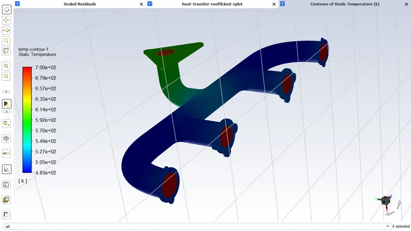
Please refer the below photo for the Temperature Contours obtained and the XY plane view. Due to the sudden bending at the outlet temperature will be decresed after that region outlet
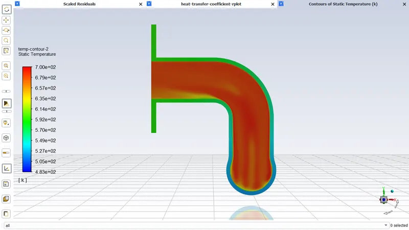
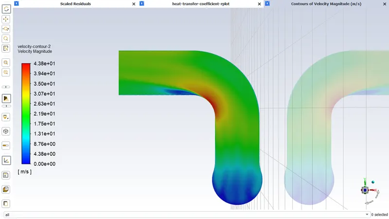
Please refer the below photo for the velocity Contours obtained and the XY plane view. Due to the sudden bending at the outlet velocity will be increased littlebit at bend and gradually velocity decreases towards outlet.
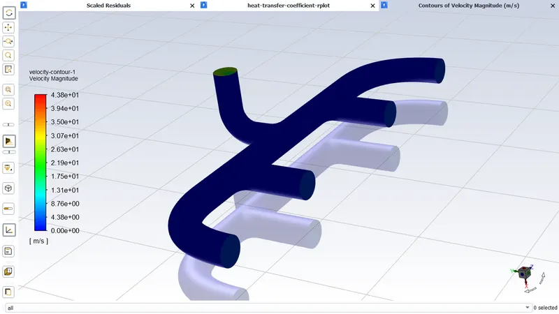
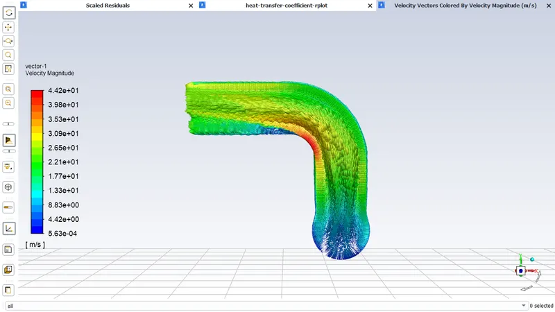
Please refer the below photo for the velocity vector obtained. Due to the sudden bending at the outlet velocity will be increased littlebit at bend and gradually velocity decreases towards outlet.
Please refer the below photo for the heat tranfer coefficient Contours obtained. From the below figure it is clear that the heat tranfer coefficient effect will be there at the fluid wall
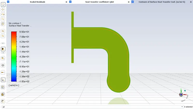
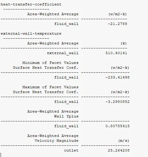
Please refer the below photo for the values obtained. The heat tranfer coefficient obtained is -21.2788 W/m2 °K at the fluid wall and external wall temperature of 510.40141°K
Case 5:
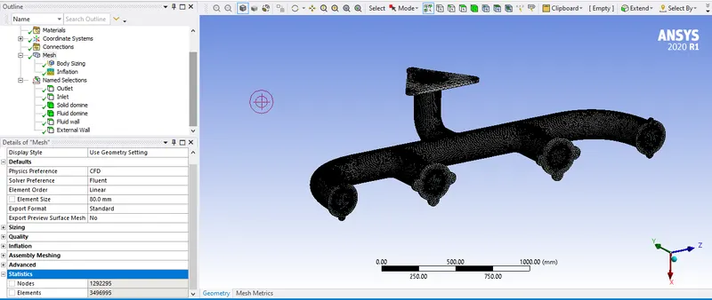
Please refer the below photo for the number of nodes and elements obtained in the case 5 is 1292295 and 3496995 respectively.
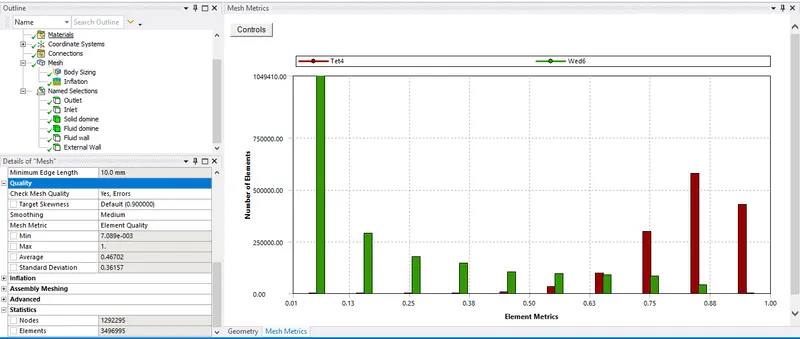
Please refer the below photo for the mesh element quality obtained , average value is 0.46702
Please refer the below photo for the mesh Skewness obtained , average value is 0.16437
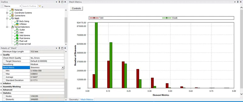
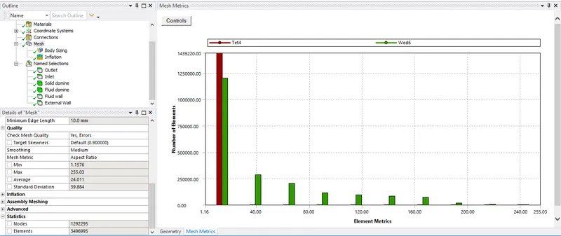
Please refer the below photo for the mesh Aspect ratio obtained , average value is 24.011
Result:
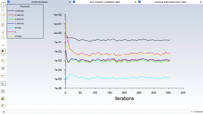
Please refer the below photo for the residuals plots obtained.
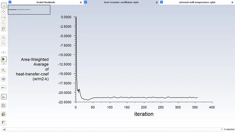
Please refer the below photo for the heat transfer coefficient plot obtained.
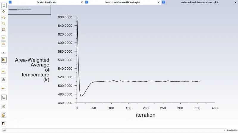
Please refer the below photo for the Temperature plot obtained.
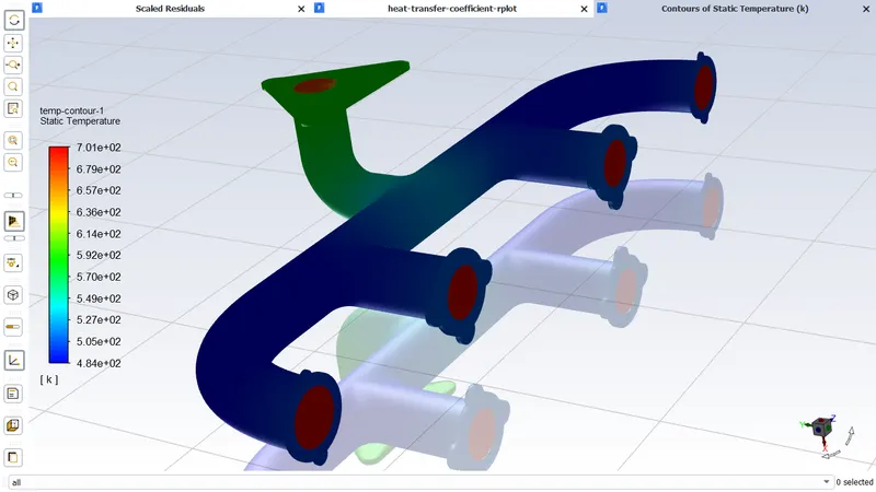
Please refer the below photo for the Temperature Contours obtained and the XY plane view. Due to the sudden bending at the outlet temperature will be decresed after that region outlet
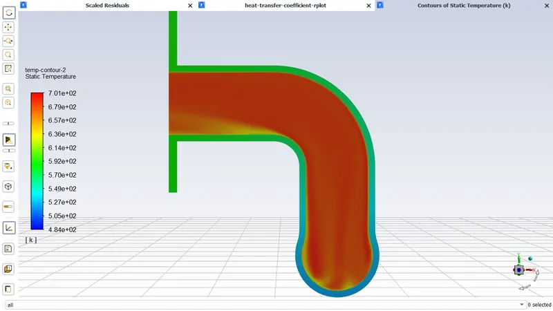
Please refer the below photo for the velocity Contours obtained and the XY plane view. Due to the sudden bending at the outlet velocity will be increased littlebit at bend and gradually velocity decreases towards outlet.
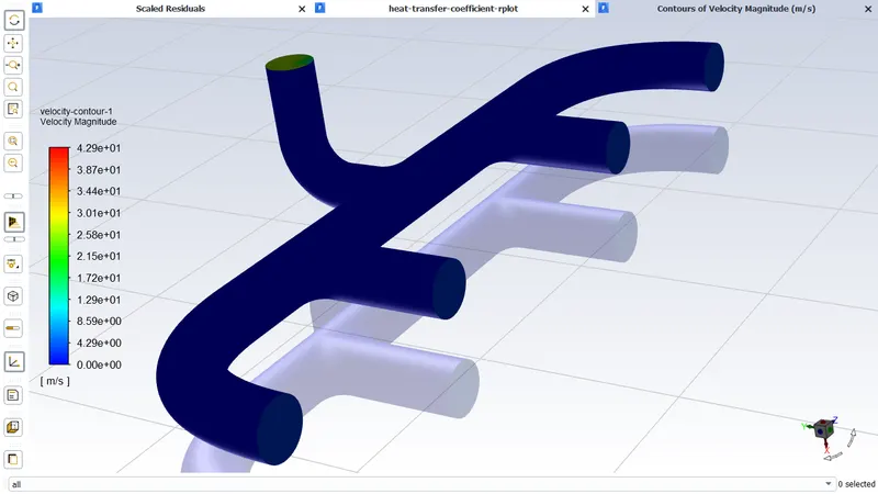
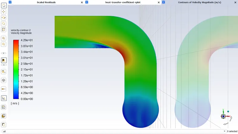
Please refer the below photo for the velocity vector obtained. Due to the sudden bending at the outlet velocity will be increased littlebit at bend and gradually velocity decreases towards outlet.
lease refer the below photo for the heat tranfer coefficient Contours obtained. From the below figure it is clear that the heat tranfer coefficient effect will be there at the fluid wall
Please refer the below photo for the values obtained. The heat tranfer coefficient obtained is -21.288611 W/m2 °K at the fluid wall and 21.288897 W/m2 °K at the fluid wall shadow, external wall temperature of 510.19351 °K
Result and conclusion:
Please refer the below table for the results obtained in all the cases.
| Case | Mesh element size for solid domine in mm | Mesh element size for Fluid domine in mm | Number of Nodes | Number of Elements | Average Element Quality | Average Aspect ratio | Average Skewness | Heat transfer coefficient near fluid wall in W/m2 °K (all are in-ve sign indicates heat rejected) | Theoritical Heat transfer coefficient near fluid wall in W/m2 °K | Error percentage Heat transfer coefficient between near wall and theoritical value | External wall temperature in °K |
| 1 | 150 | 25 | 168081 | 387485 | 0.2704 | 78.24 | 0.19897 | 21.307884 | 19.5226 | 9.144704087 | 509.89009 |
| 2 | 130 | 20 | 213880 | 498773 | 0.28228 | 70.467 | 0.18106 | 21.28897 | 19.5226 | 9.047821499 | 509. 63261 |
| 3 | 110 | 15 | 349666 | 842087 | 0.32366 | 52.917 | 0.16902 | 21.223341 | 19.5226 | 8.711652136 | 509.89296 |
| 4 | 90 | 10 | 831230 | 2167188 | 0.42168 | 31.482 | 0.16725 | 21.2788 | 19.5226 | 8.995728028 | 510.40141 |
| 5 | 80 | 8 | 1292295 | 3496995 | 0.46702 | 24.011 | 0.16437 | 21.288611 | 19.5226 | 9.045982605 | 510.19351 |
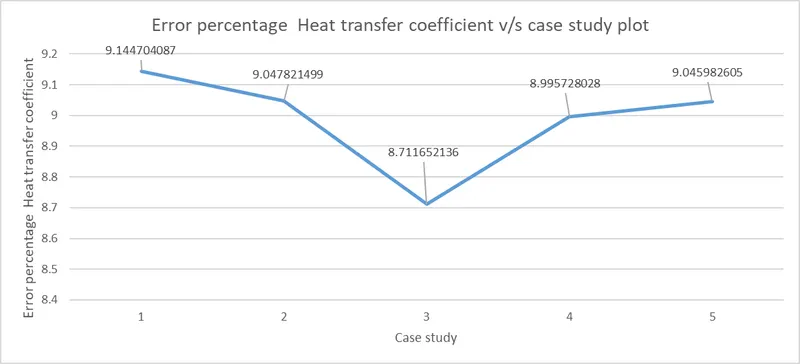
From the above graph it is confirmed that case study 3 have less Error percentage of Heat transfer coefficient between near wall and theoritical value which is preferred.
The analytical value of the heat transfer coefficient is 19.5226 W/m2 °K
The accuracy of the heat transfer coefficient depends on selecting the suitable value of Y+ and turbulence model k−ω-SST model. The heat transfer coefficient values predicted by CFD were validated against the numerical solution the deviation is within 10% which is in compliance with industrial standards. However, the accuracy of k−ω-SST model itself depends on the accuracy of the analytical solution, flow properties, and geometry.
The grid independence test was also observed during mesh refinement. The value of the heat transfer coefficient for case study 3 is near to the analytical value of the heat transfer coefficient. It is important that we limit ourselves to the case study 3 only to save the computational time and cost of the project.
.