Week 10 - Simulating Combustion of Natural Gas.

AIM & OBJECTIVES:

Part I

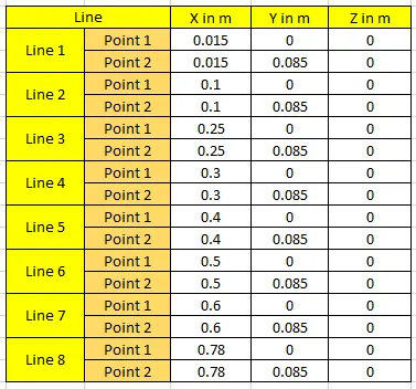
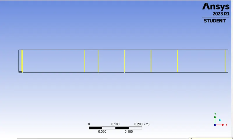
Perform a combustion simulation on the combustor model and plot the variation of the mass fraction of the different species in the simulation using line probes at different locations of the combustor as shown in Fig. Also plot for CO2, H2O, CH4, N2, O2, NOx emissions & Soot formation.

Part II

As I have observed from the above simulation, the Nox and soot is getting formed at the outlet of the combustor. Such formation has harmful effects on the environment and humans. The stringent government norms also demand the least formation of Nox and soot and to satisfy those requirements, check the effect of adding the water in the fuel.

In this part, I need to add the water content in the fuel from 5% to 30% by mole and observe the effect of it on the results. It is necessary to provide line plots and contours to prove my claim.

THEORY:

COMBUSTION:

Combustion is a complex phenomenon that is controlled by many physical processes including thermodynamics, buoyancy, chemical kinetics, radiation, mass and heat transfers and fluid mechanics. This makes conducting experiments for multi-species reacting flames extremely challenging and financially expensive. For these reasons, computer modeling of these processes is also playing a progressively important role in producing multi-scale information that is not available by using other research techniques.

Nowadays, 90% of energy is produced by combustion. For many reason, a world without combustion is unimaginable. If hypothetically combustion should stop tomorrow we would not have the energy for the entire society. In any case, it is very important to keep everything under control and manage the power of the chemical reactions. In rocket science, the combustion is essential and understanding its behaviour in profundity is one of the most important challenge for the future space exploration.

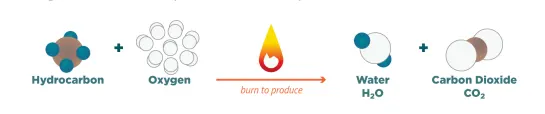
One of the main challenges regarding the combustion are surely the pollutants. Hydrocarbons CnHm are often burned and the following general reaction occurs:

When hydrocarbons are burned carbon dioxide and water cannot be avoided (main products of the chemical reaction) but the other products, the pollutants, can be avoided. The reaction of the ideal combustion is shown by the below figure is the perfect one, with maximum efficiency and no presence of pollutants, that may be reached ideally.

Thermochemistry:

Methane/pure oxygen (or air considering the nitrogen presence) combustion is treated. The main reaction as shown below is analysed in order to explain the main topic of the thermochemistry.

Air has 2 moles of oxygen + 7.52 moles of nitrogen

Mole fraction = Moles of the substance/Total moles of the mixture.

• Mole fraction of Oxygen = 2/9.52 = 0.21
• Mole fraction of Nitrogen = 7.52/9.52 = 0.79

Mass fraction:

Mass fraction = Mass of the substance / Total mass of the mixture

Mass fraction of Oxygen = (16*0.21)/((16*0.21)+(14*0.79)) = 0.23

Mass fraction of Nitrogen = (14*0.79)/((16*0.21)+(14*0.79)) = 0.76

The nitrogen does not react but it is present in the combustion reaction if air and not pure oxygen is injected. In the present project, pure liquid oxygen (LOX) is considered but sometimes particle of nitrogen are dissolved in the liquid oxygen caused by the conservation, storability method. In any case, the nitrogen is not eliminated from the simulations and, as it will be explained previously, it operates like a "bulk" quantity.

The global reaction equation without consider the presence of nitrogen is written as follows:

The stoichiometric reaction occur when 1 mole of methane reacts with 2 moles of oxygen, but what happens if less or more than 1 mole of methane for 2 moles of oxygen are present?

• If less than 1 mole of CH4 reacts with 2 moles of O2, there is oxygen left in the products because there is not enough methane to burn all the oxygen. This case is called Lean Combustion.
• The so-called Rich Combustion takes place when more than 1 mole of CH4 reacts with 2 moles of O2. Unburnt hydrocarbons are left (CO too usually) because too much methane is present within the reactants. Generally, lean is better than rich because fuel is expensive and less pollutants are produced.
The thermochemistry describes only the initial and the final states. It is totally independent of the speed at which the reaction goes from the initial to the final state.

Chemical Kinetics:

The chemical kinetics studies the speed at which chemical reactions proceed and the interest is focused on how much time this reaction needs to proceed.

In order to compute the correct value of the reaction rate, the intermediate reactions, behind the stoichiometric one, need to be taken into account. In the global reaction only the initial reactants and the final products are present. Therefore, it is possible to analyse only initial and final steps globally. In reality, between the products formation and the initial reactants many things happen and many species are created and consumed. These species that do not appear within the global reaction are called intermediate species. The reactions that describe these intermediate phenomena are called intermediate reactions. Most of them take place in the flame front, as illustrated below.

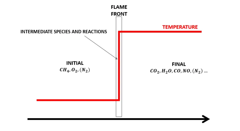
The most common tool to analyse the chemical kinetics is called Chemkin. It is a robust and mature chemistry simulation tool that has been used for a wide range of applications. Chemkin is a "cost-effective" solution for basic kinetics simulations that use small or reduced reaction mechanisms. It solves thousands of reactions combinations to develop a comprehensive understanding of a particular process, which might involve multiple chemical species, concentration ranges, and gas temperatures.

NOx formation:

The formation of NOx can be attributed to four distinct chemical kinetic processes:

Thermal NOx formation, prompt NOx formation, fuel NOx formation, and intermediate N2O.

Thermal NOx is formed by the oxidation of atmospheric nitrogen present in the combustion air.

Prompt NOx is produced by high-speed reactions at the flame front

Fuel NOx is produced by oxidation of nitrogen contained in the fuel.

At elevated pressures and oxygen-rich conditions, NOx may also be formed from molecular nitrogen (N2) via N2O.

The formation of thermal NOx is determined by a set of highly temperature dependent chemical reactions known as the extended Zeldovich mechanism. The principal reactions governing the formation of thermal NOx from molecular nitrogen are as follows:

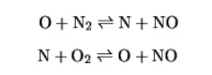
A third reaction has been shown to contribute to the formation of thermal NOx, particularly at near-stoichiometric conditions and in fuel-rich mixtures:

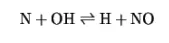
The rate of formation of NOx is significant only at high temperatures (greater than 1800 K) because fixation of nitrogen requires the breaking of the strong N2 triple bond. Also, will increase with increasing oxygen concentration. It also appears that thermal NO formation should be highly dependent on temperature but independent of fuel type. In fact, the thermal NOx production rate doubles for every 90 K temperature increase beyond 2200 K.

To evaluate the NOx formation, the concentration of O atoms and the free radical OH will be required, in addition to the concentration of stable species (i.e., O2, N2). Following the suggestion by Zeldovich, the thermal NOx formation mechanism can be decoupled from the main combustion process, by assuming equilibrium values of temperature, stable species, O atoms, and OH radicals.

Reffering to Prompt NOx, there is good evidence that can be formed in a significant quantity in some combustion environments, such as in low-temperature, fuel-rich conditions and where residence times are short.

Prompt NOx is most prevalent in rich flames. The actual formation involves a complex series of reactions and many possible intermediate species. The route is as follows:

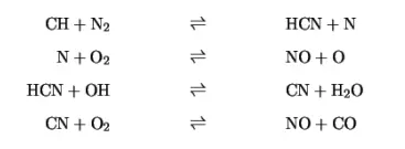
A number of species resulting from fuel fragmentation have been suggested as the source of prompt NOx in hydrocarbon flames (e.g., CH, CH2, C, C2H), but the major contribution is from CH2 via:

The other two mechanisms won’t have an effect on the NOx formation of this study because, the fuel NOx are associated to Nitrogenized hydrocarbons (not presents as the fuel is pure methane) and the NO2 intermediate mechanism is associated to high pressure systems.

Species Transport Approach

Convection, diffusion, and reaction sources conservation equations for many component species are solved using this method. Multiple chemical processes that occur in the bulk flow, at wall or particle surfaces, or in the porous zone can all be specified by the user for modeling at the same time.

Multicomponent transport inevitably introduces several important physical effects into the system, such as temperature gradients, enthalpy transmission, and diffusion.

• Finite-Rate model (Arrhenius kinetics)

General finite-rate chemistry directly determines reaction rates by ignoring the impact of turbulent fluctuations on kinetics rates.

• Eddy-dissipation model

To avoid costly Arrhenius chemical kinetic calculations, reaction rates are believed to be controlled by turbulence while neglecting the impact of chemistry timeframes. The model is computationally cheap, but only one or two-step heat-release mechanisms should be utilized for realistic results. This strategy should only be applied when the chemistry timescales of interest are known to be quick compared to the domain’s turbulence timescales.

• Eddy-dissipation-concept model

Turbulent flames can incorporate complicated chemical kinetics while considering turbulence and kinetics timescales. It should be noted that detailed simulations of chemical kinetics might be computationally expensive.

Diffusion- or kinetics-limited surface reactions are also possible; in the second case, surface coverage may also be important. In this situation, Fluent can monitor the molar concentrations of species that have adsorption to walls. Modeling of particle surface reactions is also possible.

Combustion stimulation Types:

1. Based on Mixing:

• Non-premixed combustion(Direct injection, Late injection)
• Premixed combustion (Carburetor)
• Partially premixed.

2. Based on phase

• Fluid phase (Volumetric reactions)
• Wall (Surface reactions)
• Particles (Surface reaction)
• Porous region.

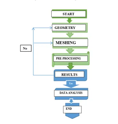
Please refer the below chart for the CFD work flow analysis of the combustion simulation on the combustor model.

Geometry Set-up:

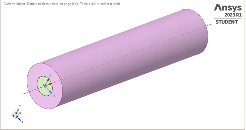
Please refer the below photo for the Geometry imported.

Please refer the below photo for the split body applied by creating the respective plane.

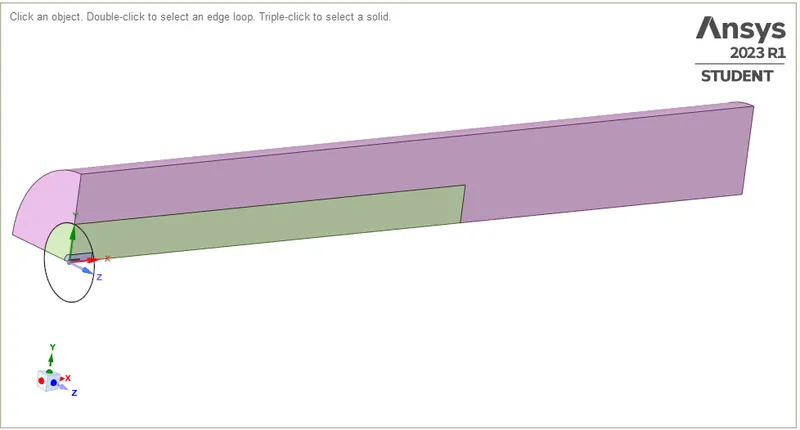
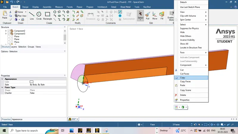
Please refer the below photo for the region copy to get the 2D geometry.

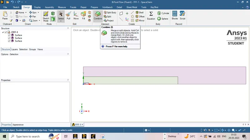
Please refer the below photo for the 2D geometry obtained.

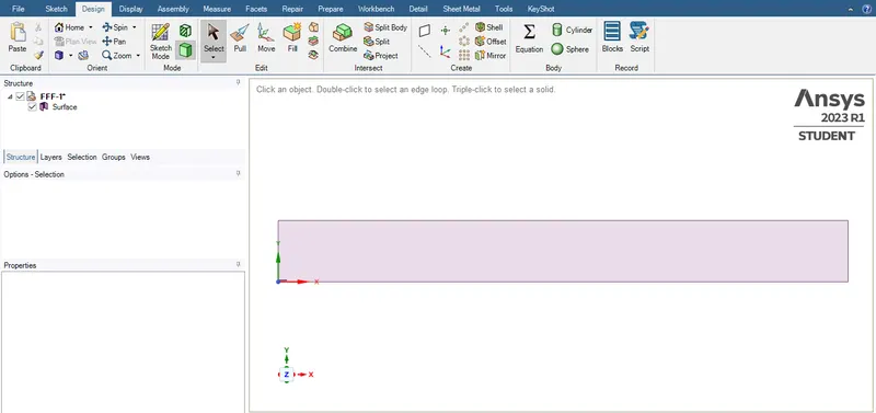
Please refer the below photo for the single surface obtained by using combine comand.

Meshing Set-up:

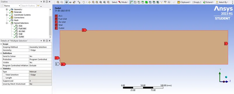
Please refer the below photo for the nomenclature of the model as Axis, Fuel inlet , Air inlet, Wall and Outlet.

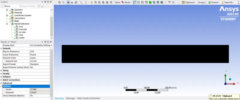
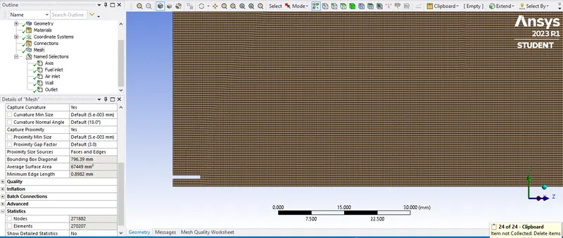
Please refer the below photo for the mesh obtained. No of nodes obtained is 271882 and No of Elements obtained is 270207.

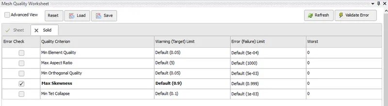
Please refer the below photo for the Quality mesh sheet obtained.

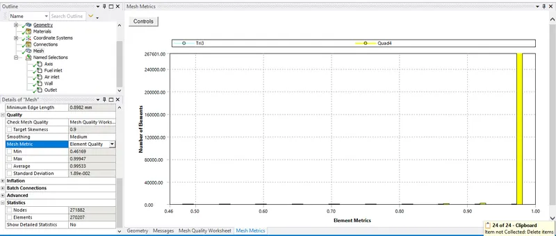
Please refer the below photo for the element quality obtained and the average value is 0.99533

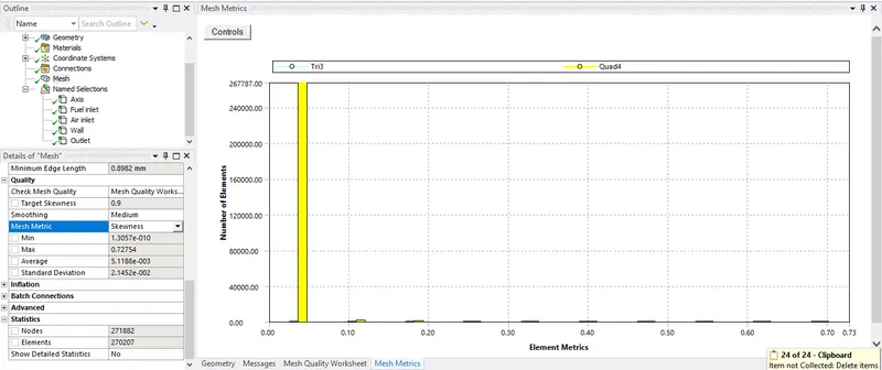
Please refer the below photo for the Skewness obtained and the average value is 5.1188e-003

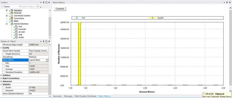
Please refer the below photo for the Aspect ratio obtained and the average value is 1.0051

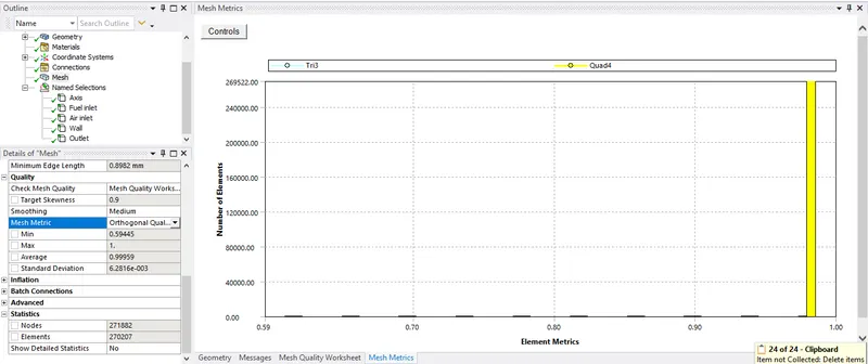
Please refer the below photo for the Ortogonal quality obtained and the average value is 0.99959

Pre-processing or Fluent Set-up:

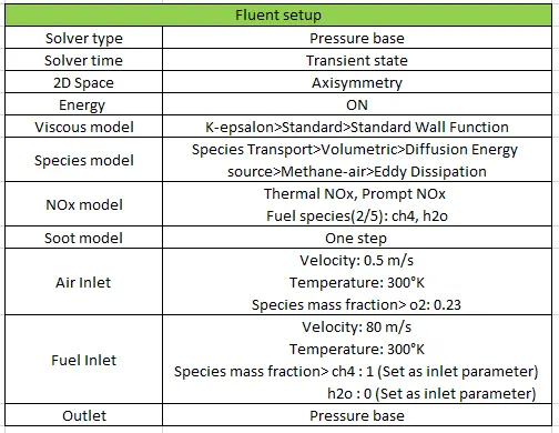
Please refer the below table for the Fluent Set-up applied.

Please refer the below photo for the Solver type applied.

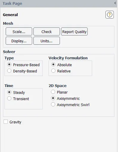
Please refer the below photo for the energy on applied.

Please refer the below photo for the Viscous model applied.

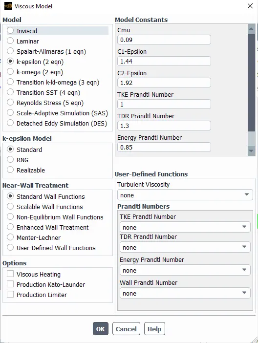
Please refer the below photo for the Species model applied.

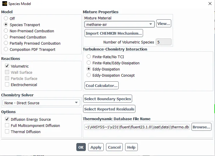
Please refer the below photo for the NOx model applied.

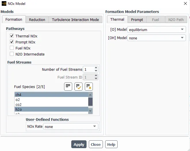
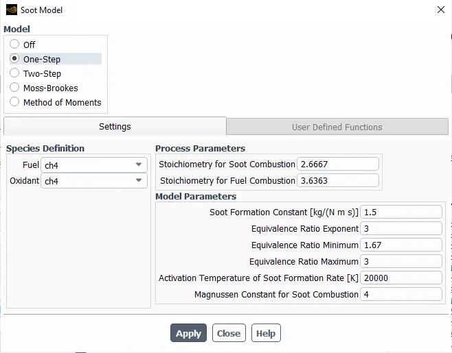
Please refer the below photo for the Soot model applied.

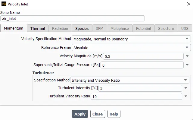
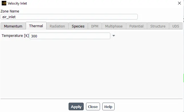
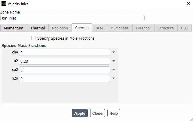
Please refer the below photo for the Air Inlet Veolcity, Thermal and Species applied.

Please refer the below photo for the Fuel Inlet Veolcity, Thermal and Species parameter applied.

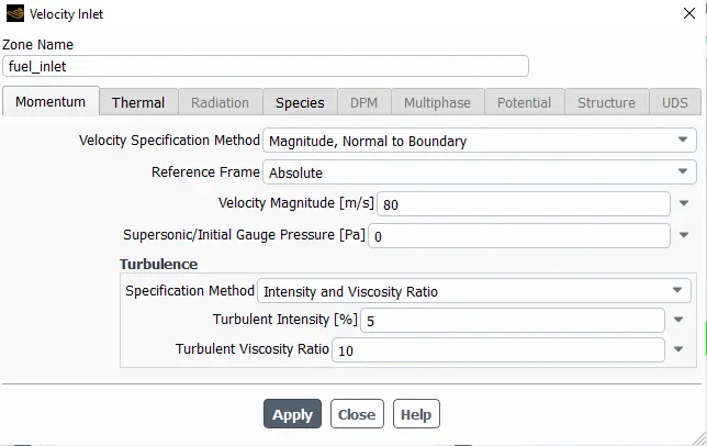
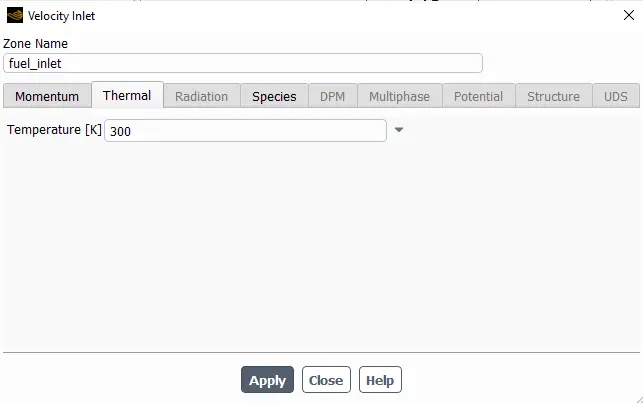
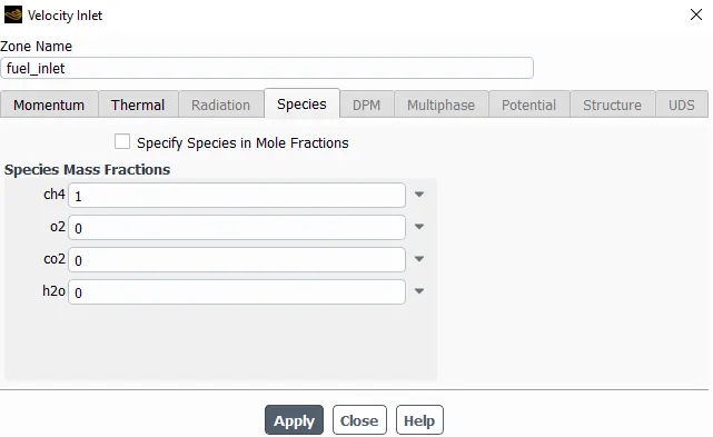
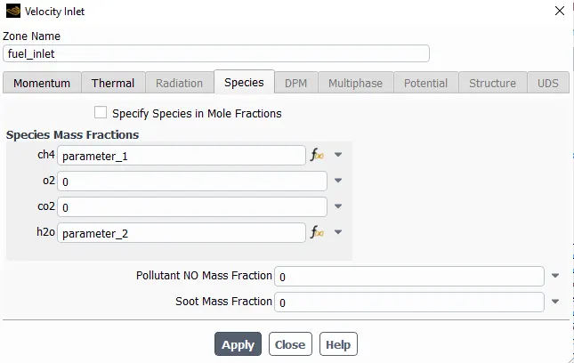
Please refer the below photo for the Report defination applied and Input and output parameter.

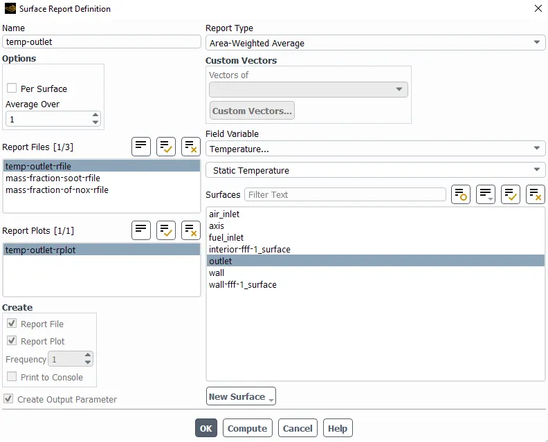
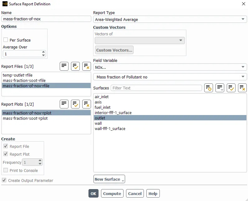
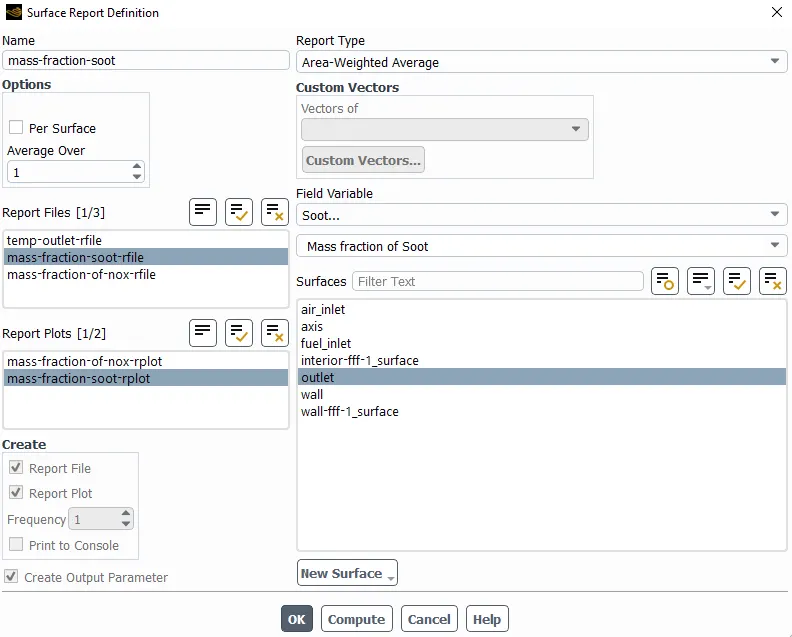
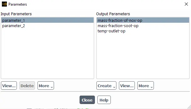
After applying the inlet parameters Hybrid initialization done and run for 1000 itiration in Run Calculation.

Results and Post-Processing Set-up:

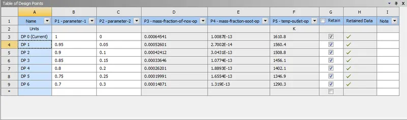
Please refer the below table for the Parameter table obtained.

Please refer the below table for the 8 line and their points applied.

Please refer the below photo for the 8 line applied.

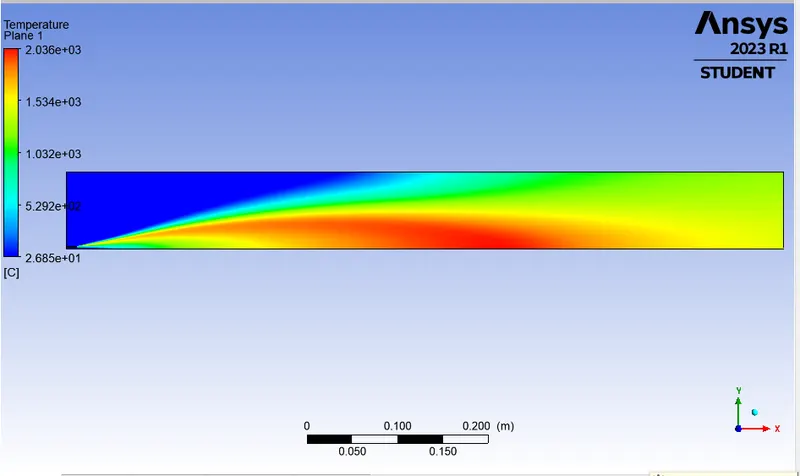
Case 1 : 100% Methane and 0% Water

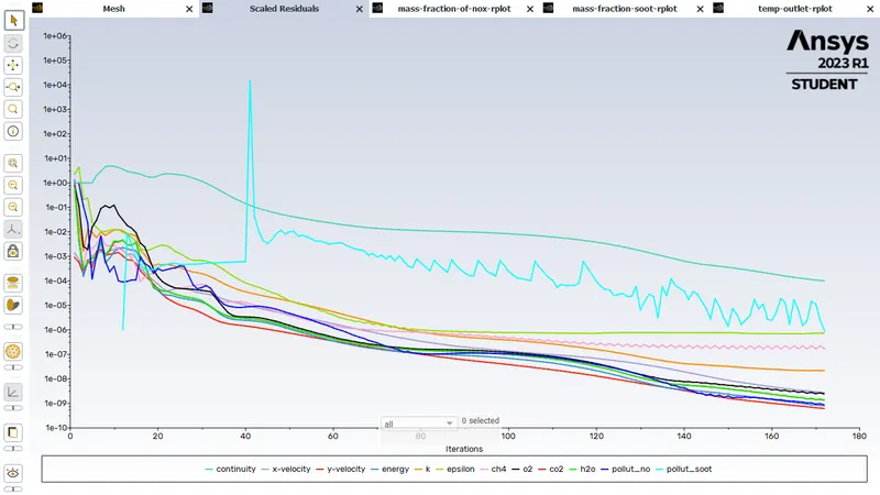
Please refer the below photo for the Residuals obtained.

Please refer the below photo for the Temperature plot obtained.

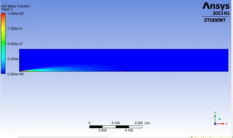
Please refer the below photo for the CH4 Mass fraction plot obtained.

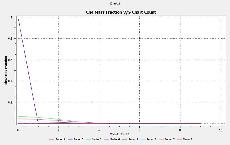
Please refer the below photo for the CH4 Mass fraction Chart obtained.

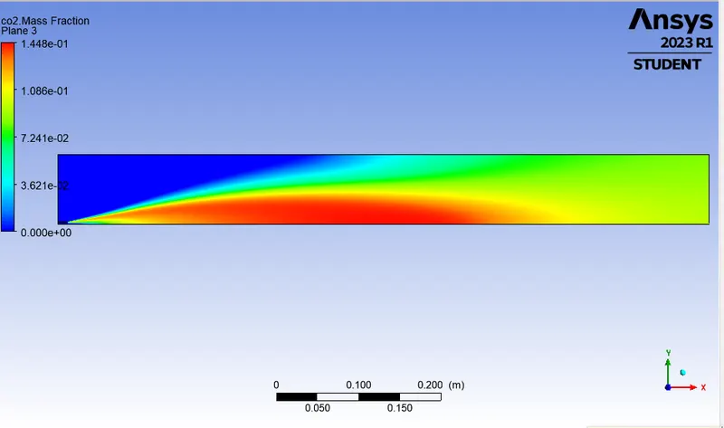
Please refer the below photo for the CO2 Mass fraction plot obtained.

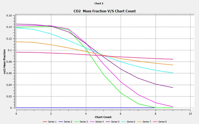
Please refer the below photo for the CO2 Mass fraction Chart obtained.

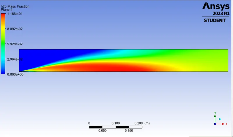
Please refer the below photo for the H20 Mass fraction plot obtained.

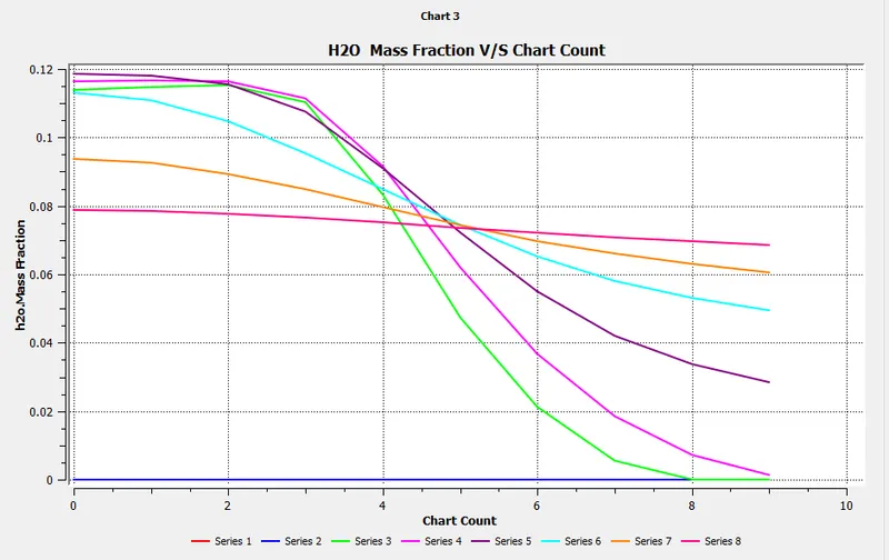
Please refer the below photo for the H20 Mass fraction Chart obtained.

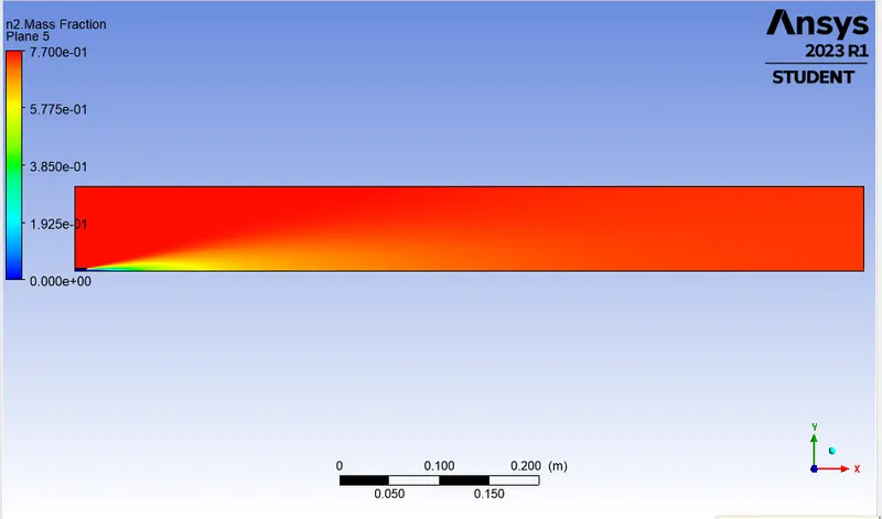
Please refer the below photo for the N2 Mass fraction plot obtained.

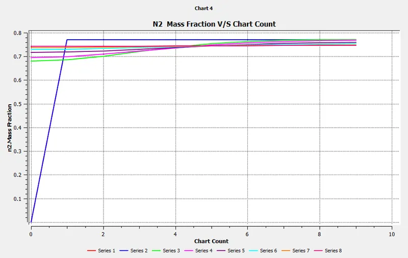
Please refer the below photo for the N2 Mass fraction Chart obtained.

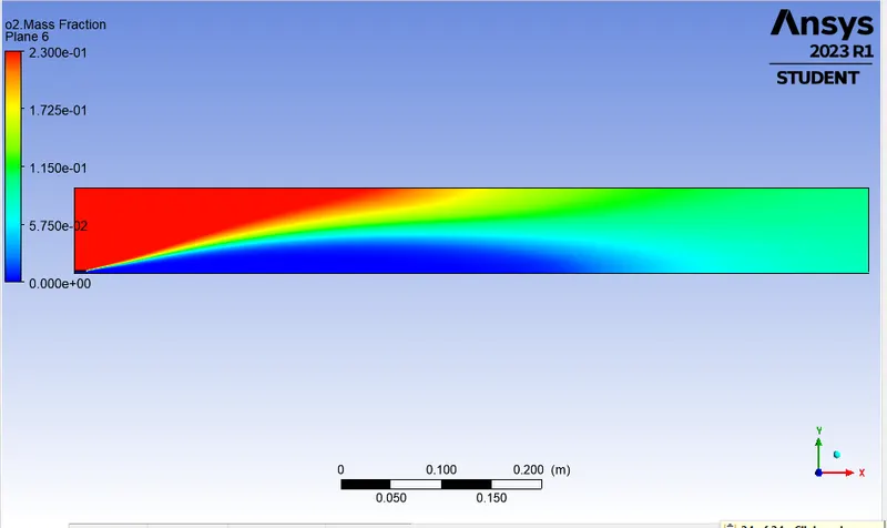
Please refer the below photo for the O2 Mass fraction plot obtained.

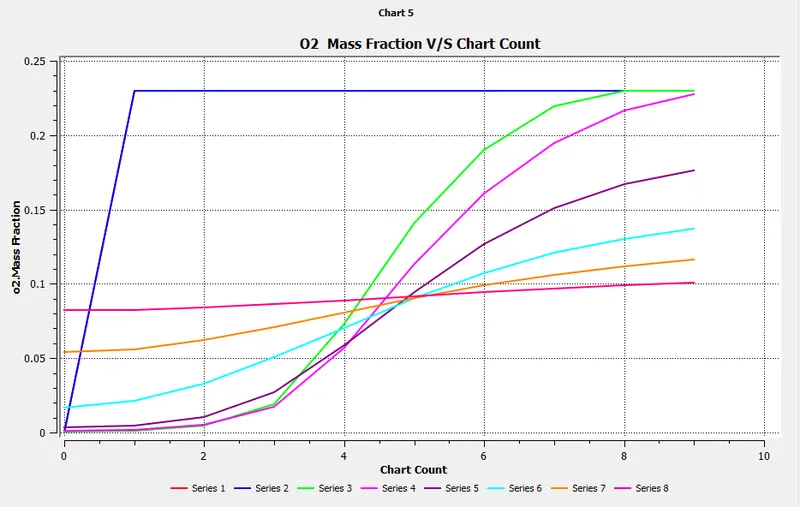
Please refer the below photo for the O2 Mass fraction Chart obtained.

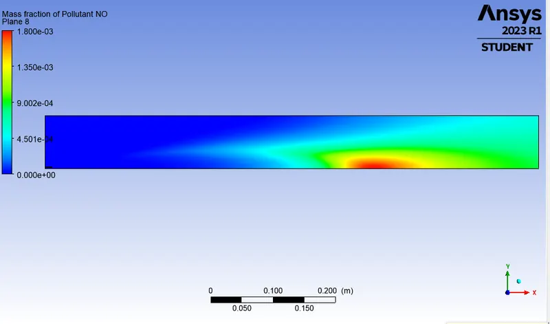
Please refer the below photo for the NO Mass fraction of pollutent plot obtained.

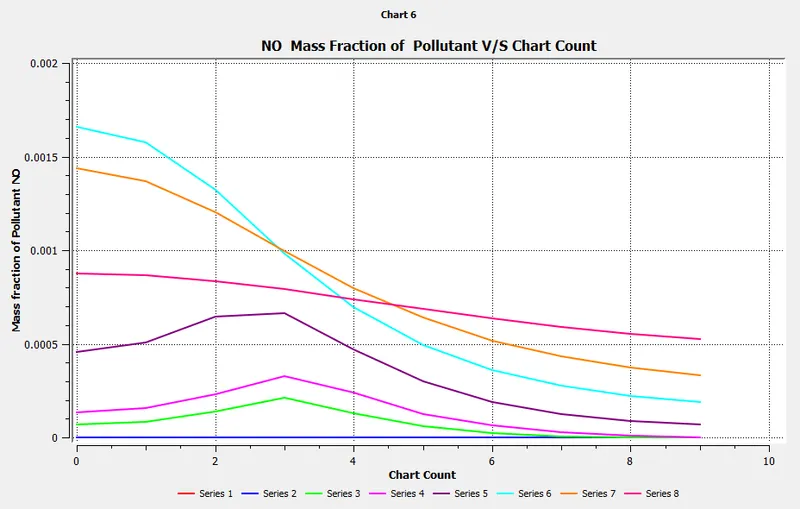
Please refer the below photo for the NO Mass fraction of pollutent Chart obtained.

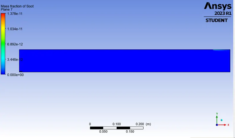
Please refer the below photo for the Mass fraction of Soot plot obtained.

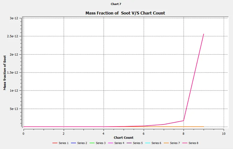
Please refer the below photo for the Mass fraction of Soot Chart obtained.

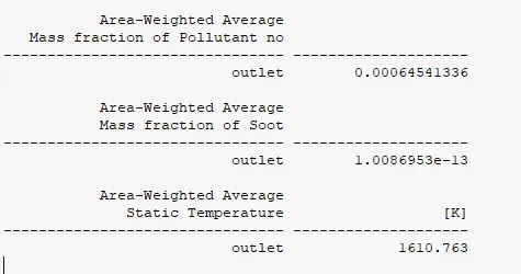
Please refer the below photo for the results obtained.

Case 2 : 95% Methane and 5% Water

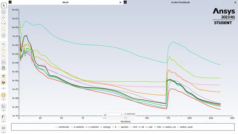
Please refer the below photo for the Residuals obtained.

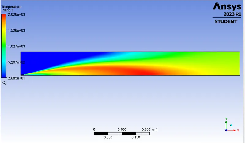
Please refer the below photo for the Temperature plot obtained.

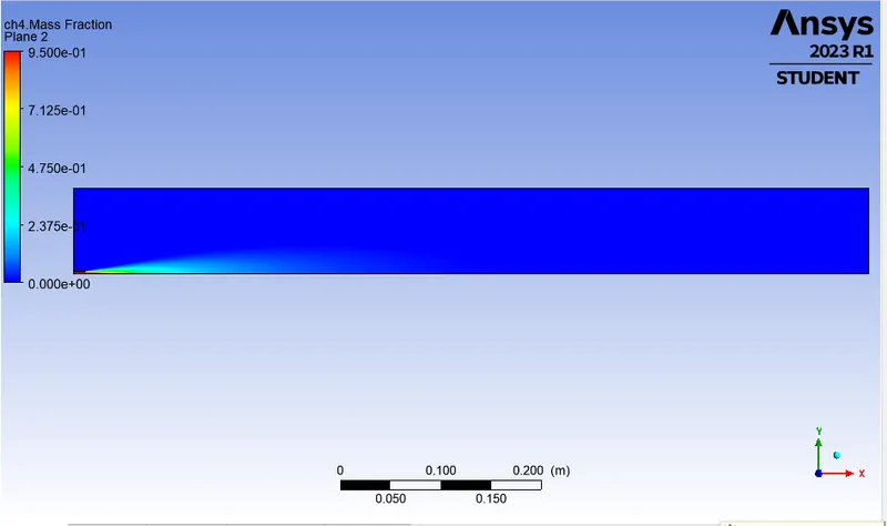
Please refer the below photo for the CH4 Mass fraction plot obtained.

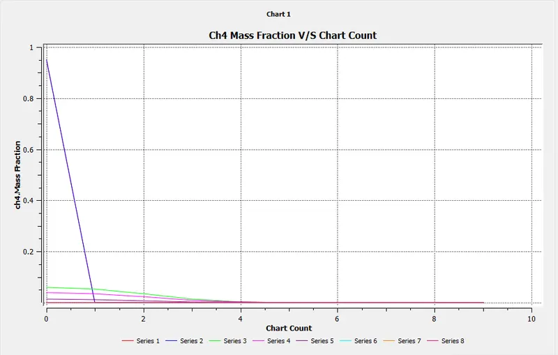
Please refer the below photo for the CH4 Mass fraction Chart obtained.

Please refer the below photo for the CO2 Mass fraction plot obtained.

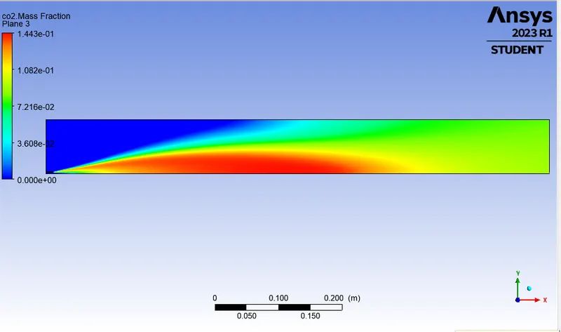
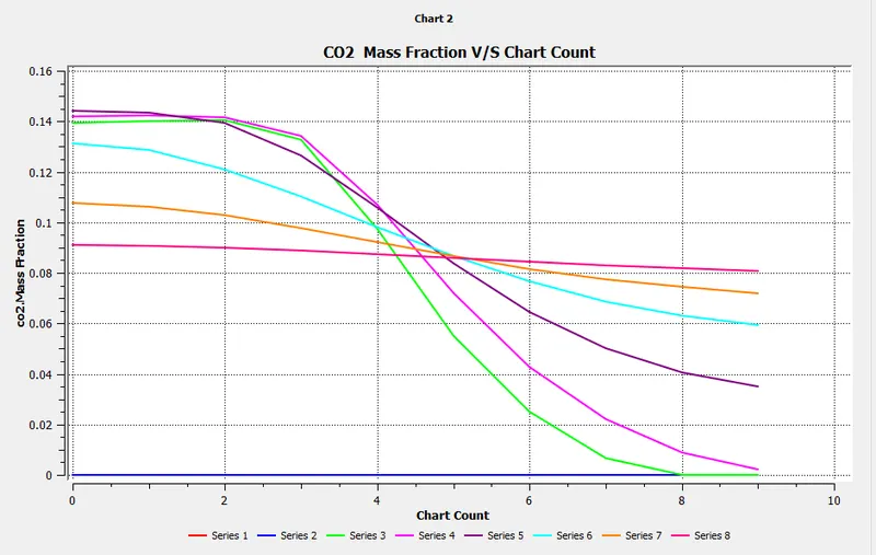
Please refer the below photo for the CO2 Mass fraction Chart obtained.

Please refer the below photo for the H20 Mass fraction plot obtained.

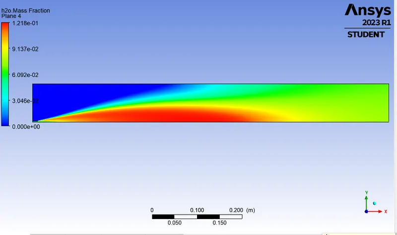
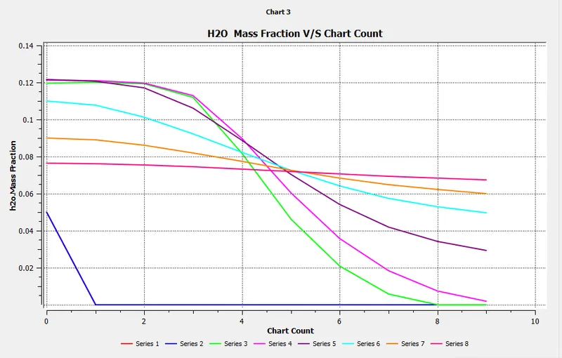
Please refer the below photo for the H20 Mass fraction Chart obtained.

Please refer the below photo for the N2 Mass fraction plot obtained.

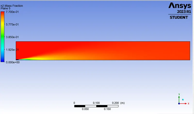
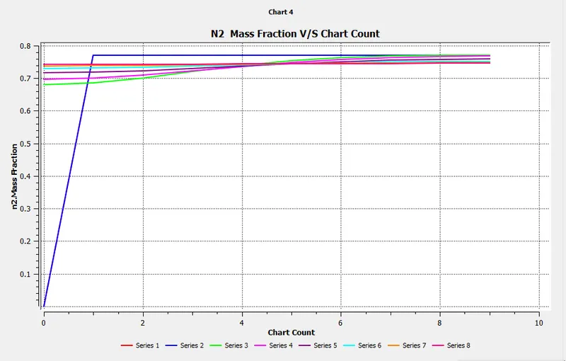
Please refer the below photo for the N2 Mass fraction Chart obtained.

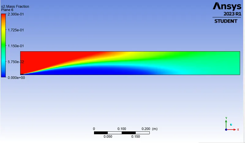
Please refer the below photo for the O2 Mass fraction plot obtained.

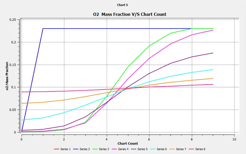
Please refer the below photo for the O2 Mass fraction Chart obtained.

Please refer the below photo for the NO Mass fraction of pollutent plot obtained.

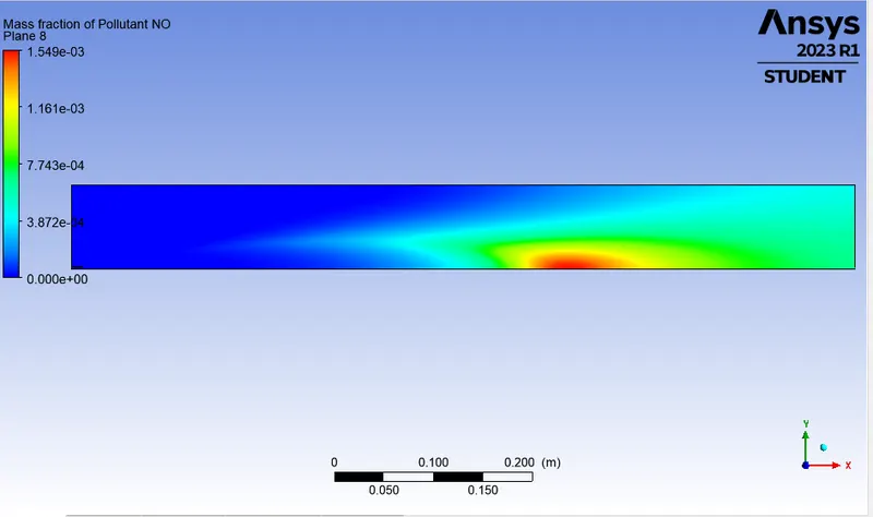
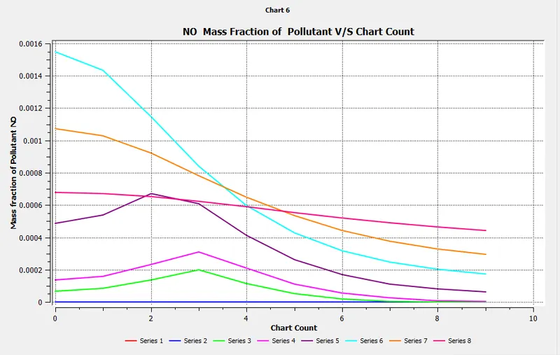
Please refer the below photo for the NO Mass fraction of pollutent Chart obtained.

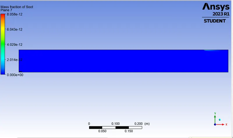
Please refer the below photo for the Mass fraction of Soot plot obtained.

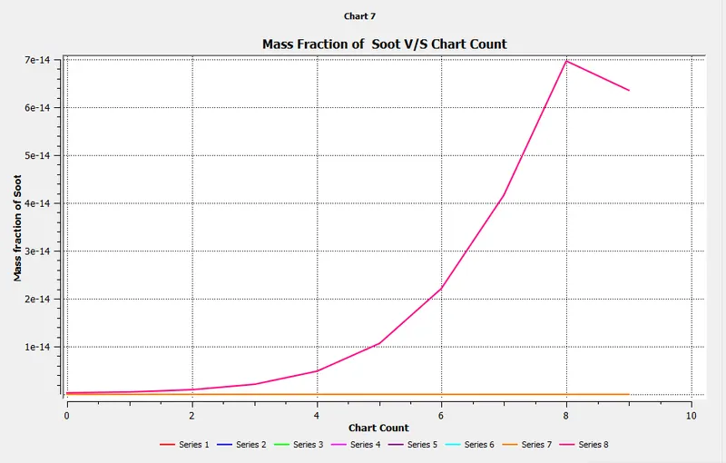
Please refer the below photo for the Mass fraction of Soot Chart obtained.

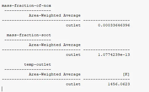
Please refer the below photo for the results obtained.

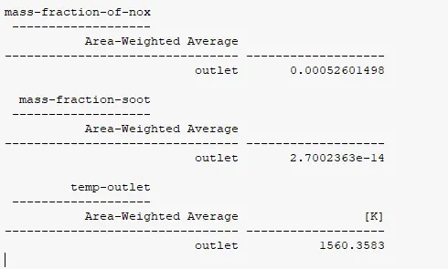
Case 3 : 90% Methane and 10% Water

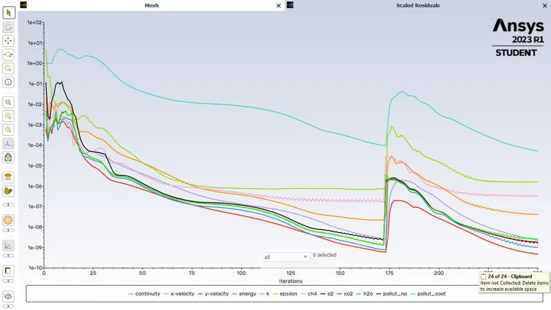
Please refer the below photo for the Residuals obtained.

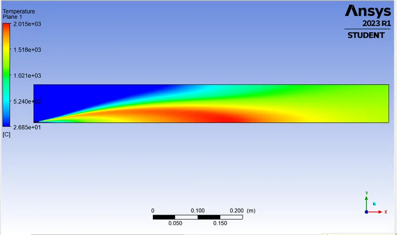
Please refer the below photo for the Temperature plot obtained.

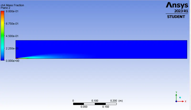
Please refer the below photo for the CH4 Mass fraction plot obtained.

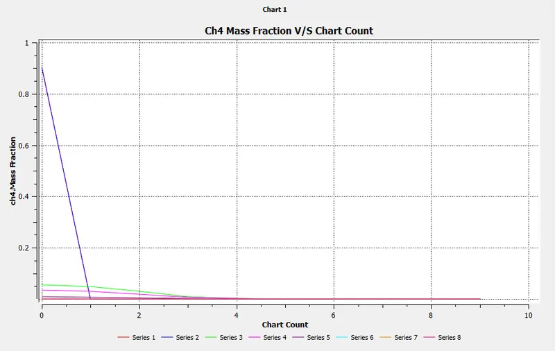
Please refer the below photo for the CH4 Mass fraction Chart obtained.

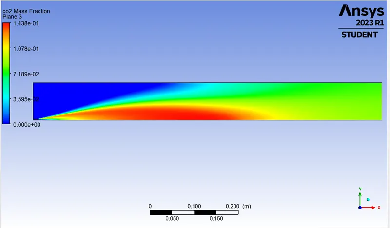
Please refer the below photo for the CO2 Mass fraction plot obtained.

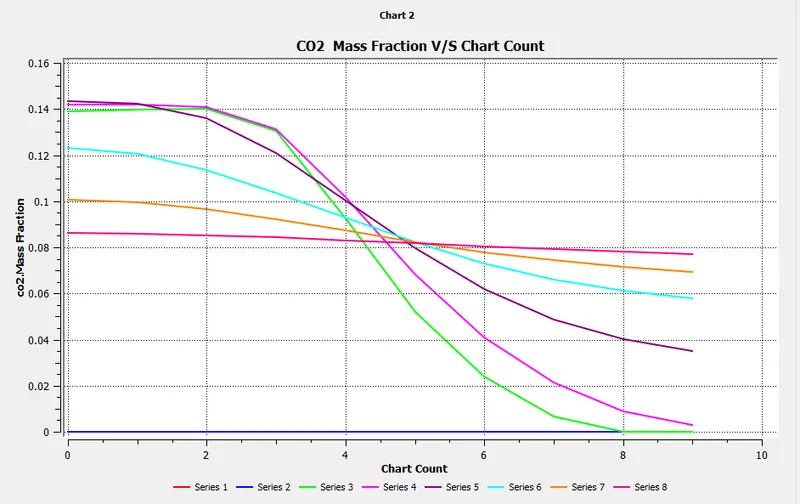
Please refer the below photo for the CO2 Mass fraction Chart obtained.

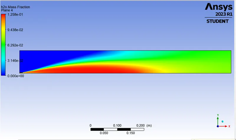
Please refer the below photo for the H20 Mass fraction plot obtained.

Please refer the below photo for the H20 Mass fraction Chart obtained.

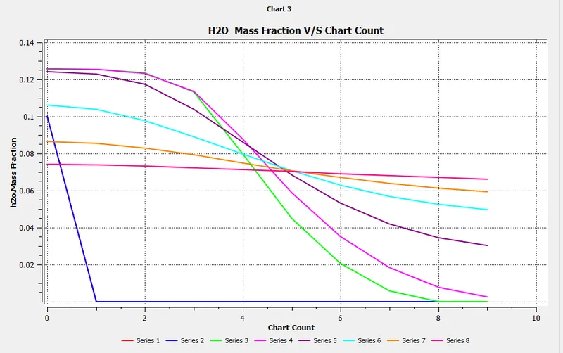
Please refer the below photo for the N2 Mass fraction plot obtained.

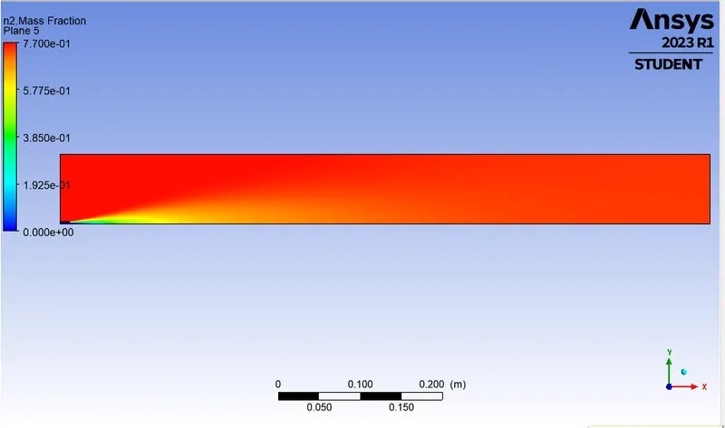
Please refer the below photo for the N2 Mass fraction Chart obtained.

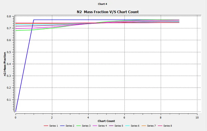
Please refer the below photo for the O2 Mass fraction plot obtained.

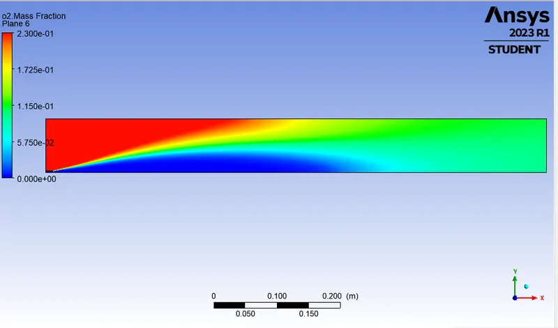
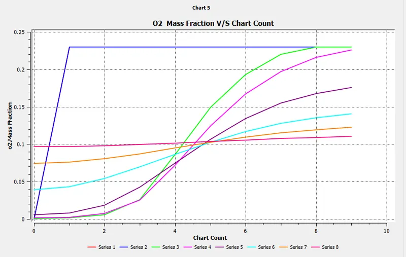
Please refer the below photo for the O2 Mass fraction Chart obtained.

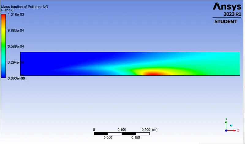
Please refer the below photo for the NO Mass fraction of pollutent plot obtained.

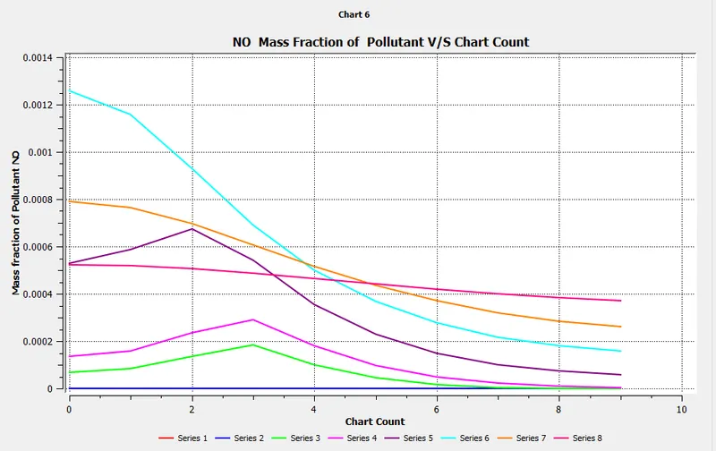
Please refer the below photo for the NO Mass fraction of pollutent Chart obtained.

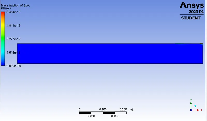
Please refer the below photo for the Mass fraction of Soot plot obtained.

Please refer the below photo for the Mass fraction of Soot Chart obtained.

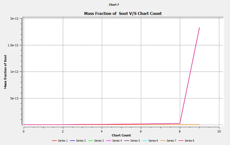
Please refer the below photo for the results obtained.

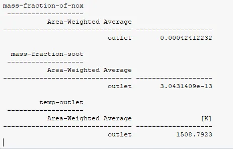
Case 4 : 85% Methane and 15% Water

Please refer the below photo for the Residuals obtained.

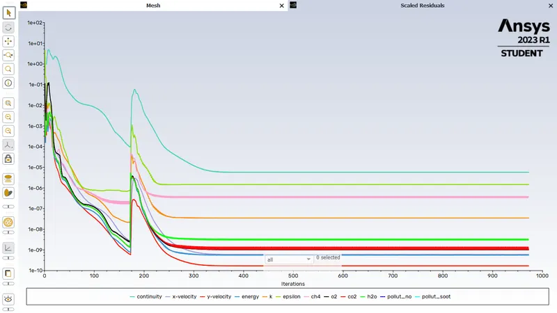
Please refer the below photo for the Temperature plot obtained.

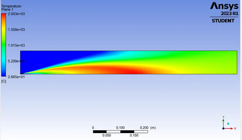
Please refer the below photo for the CH4 Mass fraction plot obtained.

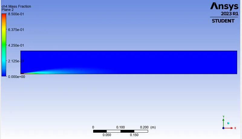
Please refer the below photo for the CH4 Mass fraction Chart obtained.

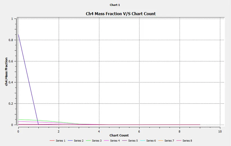
Please refer the below photo for the CO2 Mass fraction plot obtained.

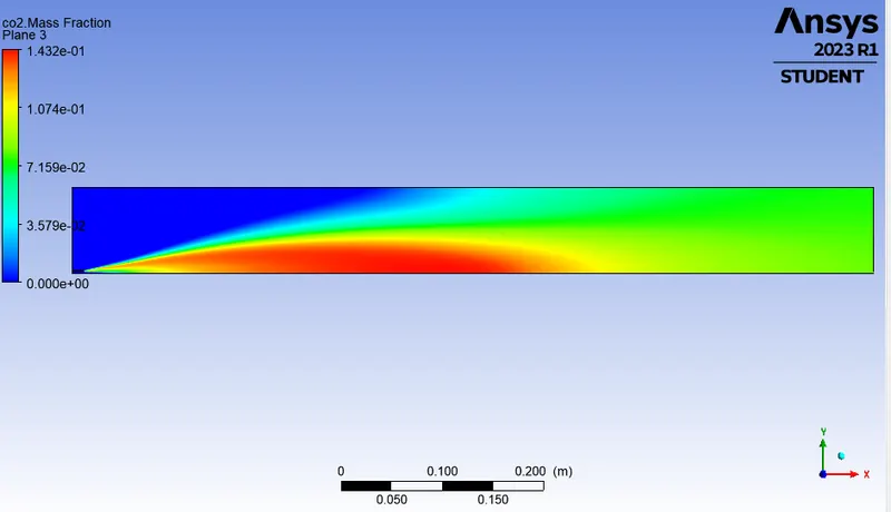
Please refer the below photo for the CO2 Mass fraction Chart obtained.

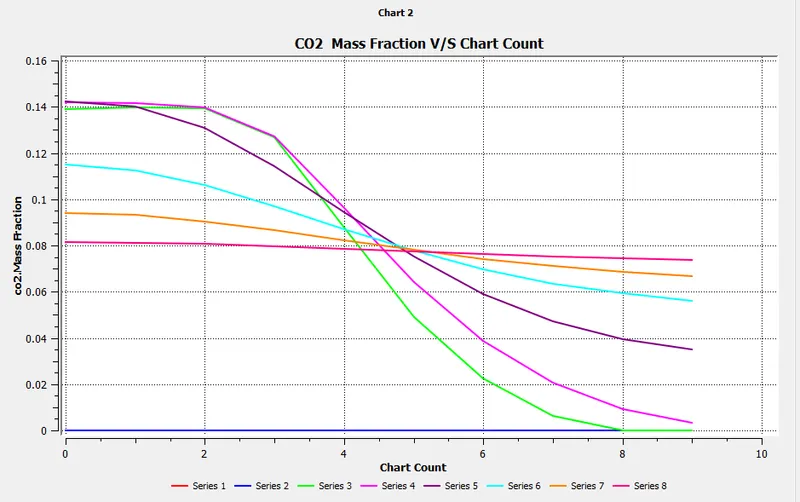
Please refer the below photo for the H20 Mass fraction plot obtained.

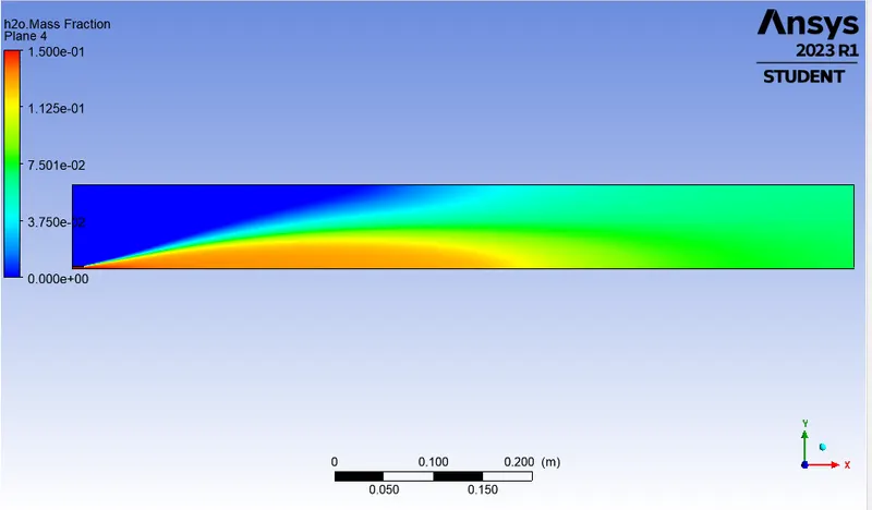
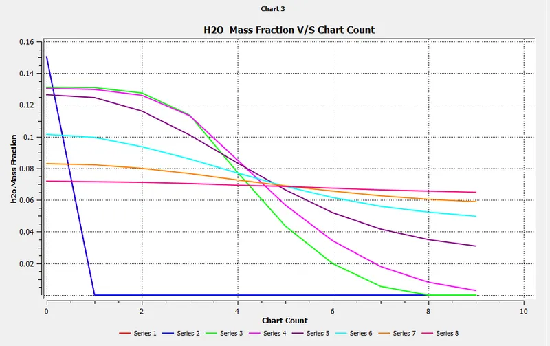
Please refer the below photo for the H20 Mass fraction Chart obtained.

Please refer the below photo for the N2 Mass fraction plot obtained.

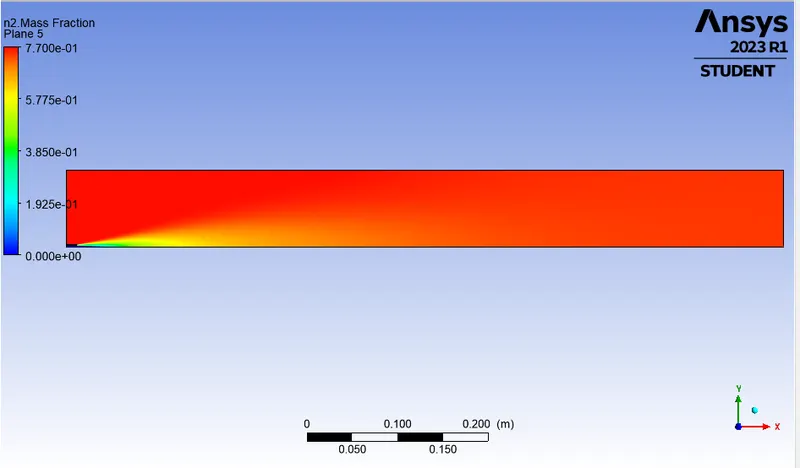
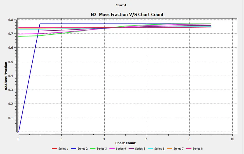
Please refer the below photo for the N2 Mass fraction Chart obtained.

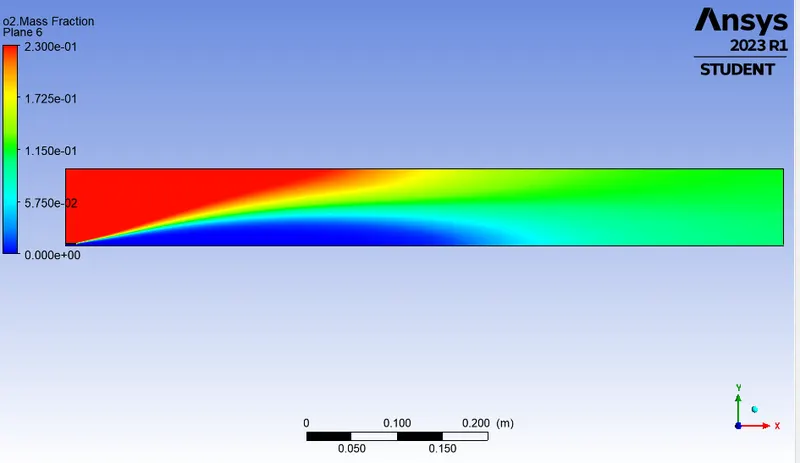
Please refer the below photo for the O2 Mass fraction plot obtained.

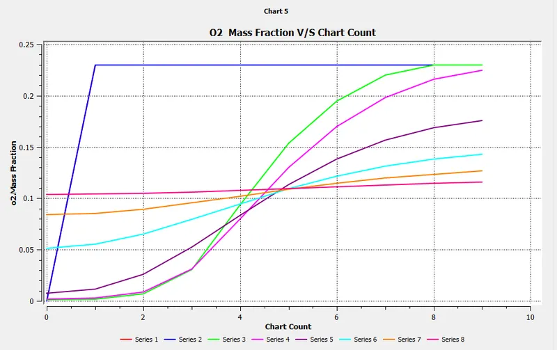
Please refer the below photo for the O2 Mass fraction Chart obtained.

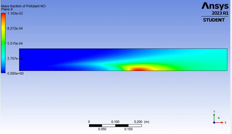
Please refer the below photo for the NO Mass fraction of pollutent plot obtained.

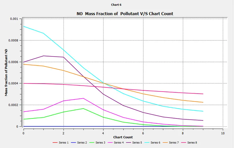
Please refer the below photo for the NO Mass fraction of pollutent Chart obtained.

Please refer the below photo for the Mass fraction of Soot plot obtained.

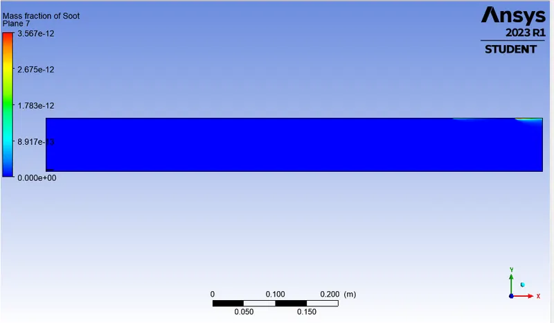
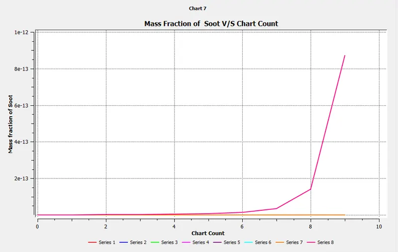
Please refer the below photo for the Mass fraction of Soot Chart obtained.

Please refer the below photo for the results obtained.

Case 5 : 80% Methane and 20% Water

Please refer the below photo for the Residuals obtained.

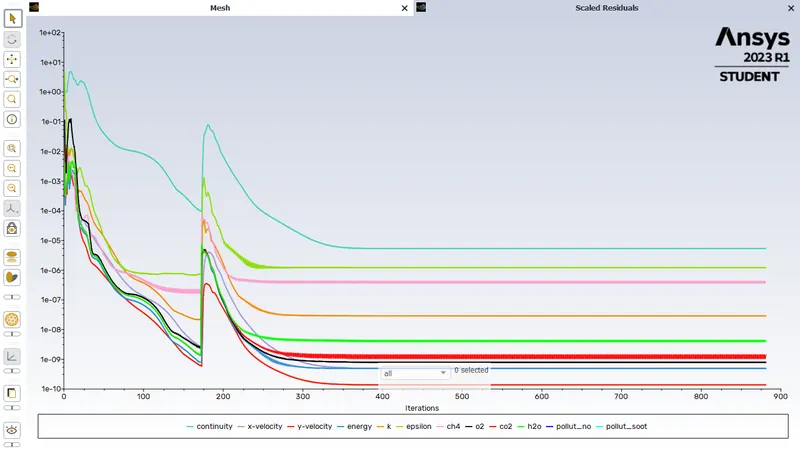
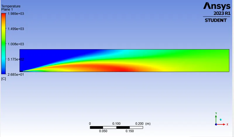
Please refer the below photo for the Temperature plot obtained.

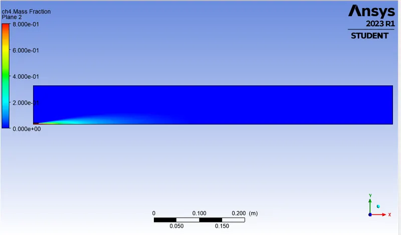
Please refer the below photo for the CH4 Mass fraction plot obtained.

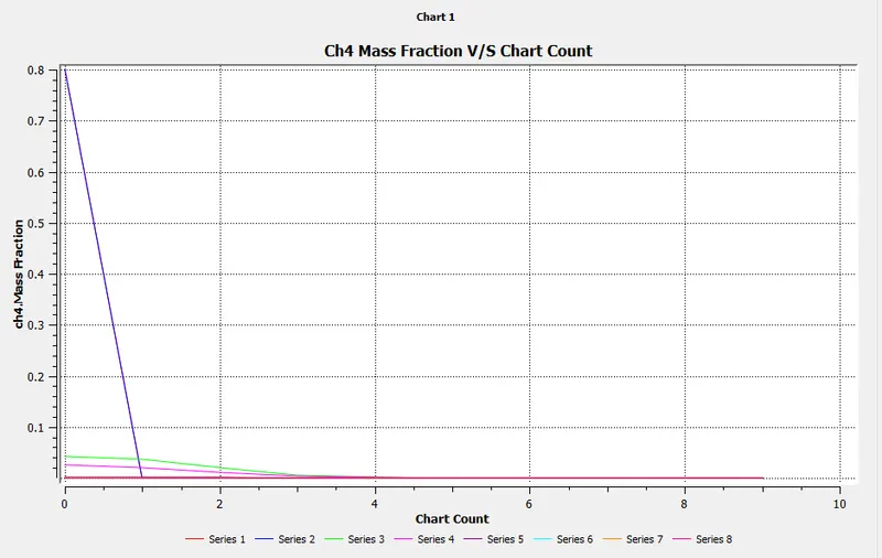
Please refer the below photo for the CH4 Mass fraction Chart obtained.

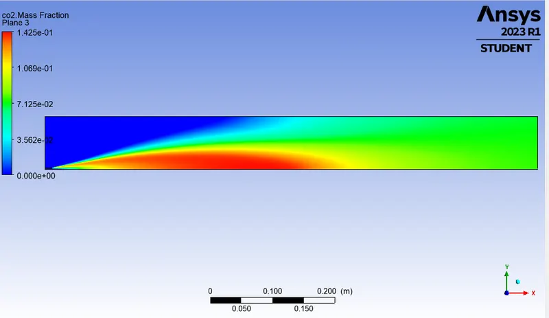
Please refer the below photo for the CO2 Mass fraction plot obtained.

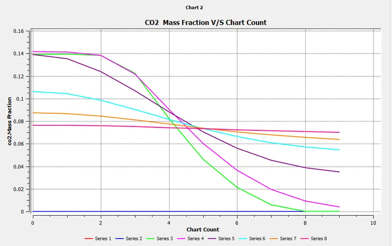
Please refer the below photo for the CO2 Mass fraction Chart obtained.

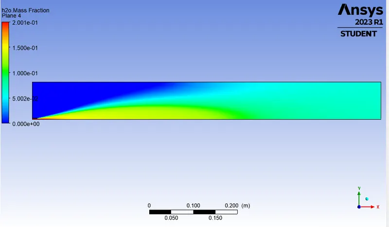
Please refer the below photo for the H20 Mass fraction plot obtained.

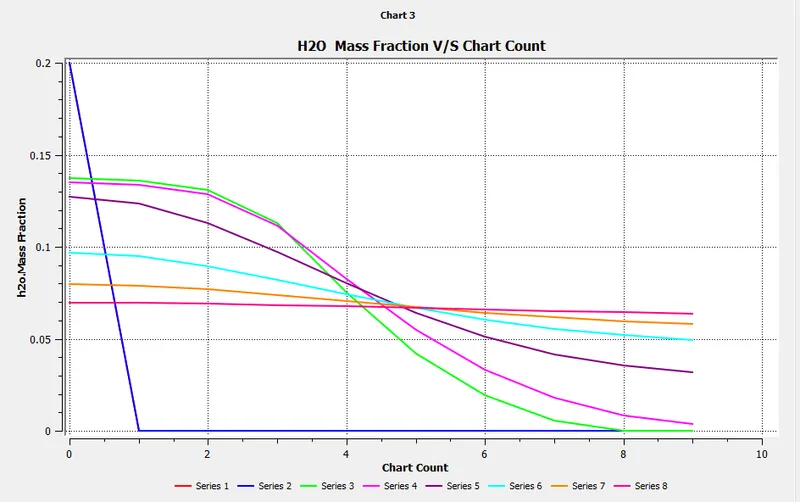
Please refer the below photo for the H20 Mass fraction Chart obtained.

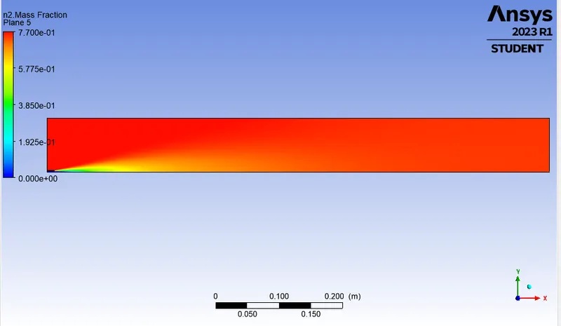
Please refer the below photo for the N2 Mass fraction plot obtained.

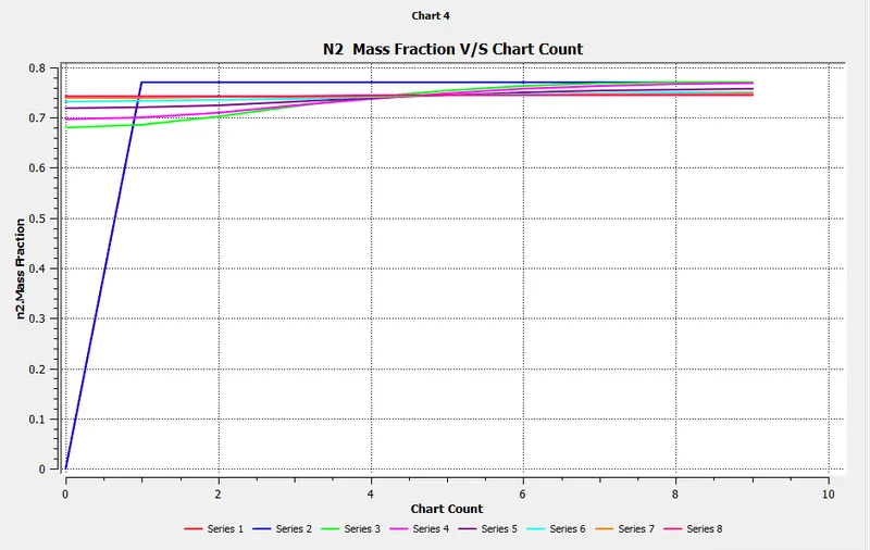
Please refer the below photo for the N2 Mass fraction Chart obtained.

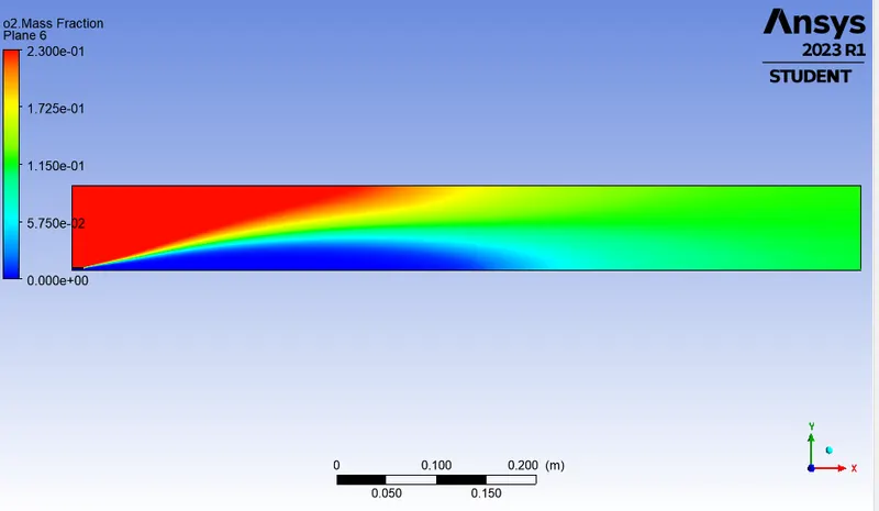
Please refer the below photo for the O2 Mass fraction plot obtained.

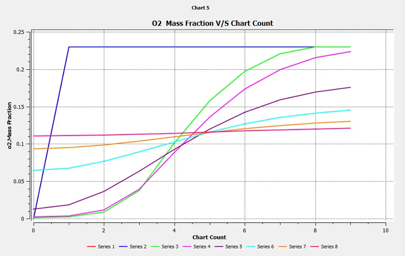
Please refer the below photo for the O2 Mass fraction Chart obtained.

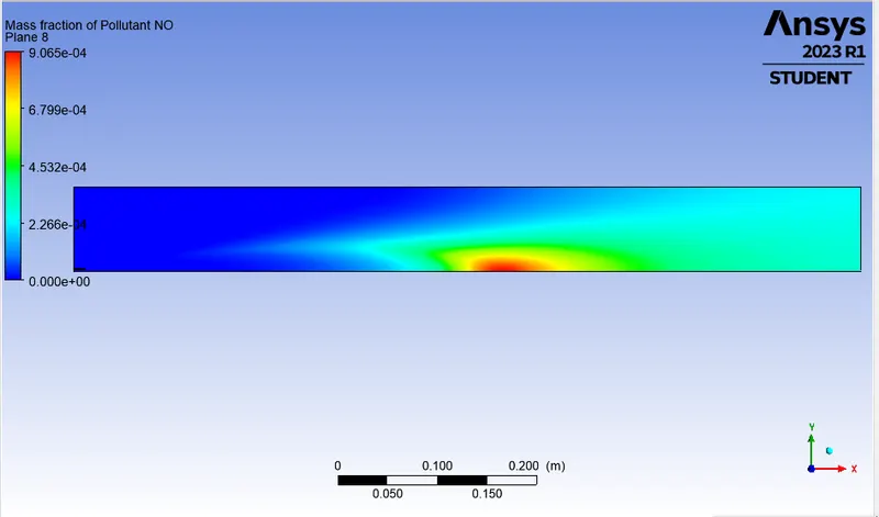
Please refer the below photo for the NO Mass fraction of pollutent plot obtained.

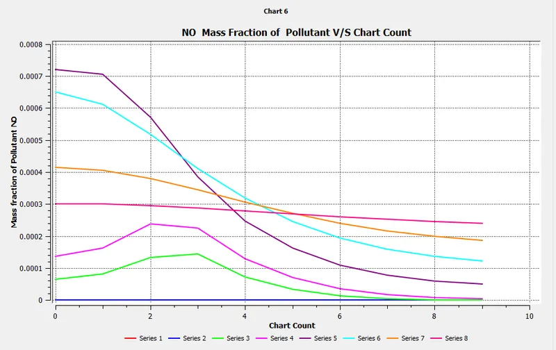
Please refer the below photo for the NO Mass fraction of pollutent Chart obtained.

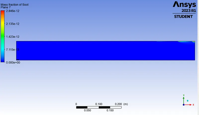
Please refer the below photo for the Mass fraction of Soot plot obtained.

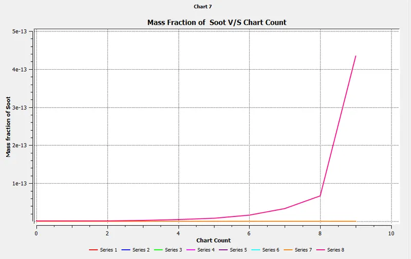
Please refer the below photo for the Mass fraction of Soot Chart obtained.

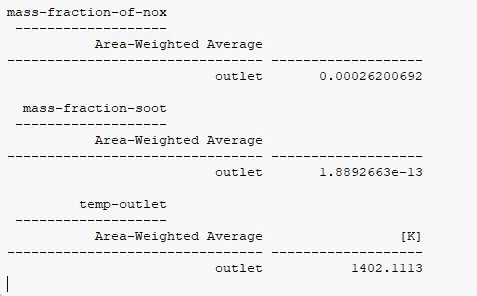
Please refer the below photo for the results obtained.

Case 6 : 75% Methane and 25% Water

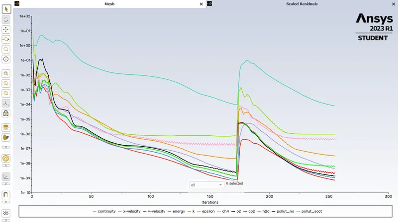
Please refer the below photo for the Residuals obtained.

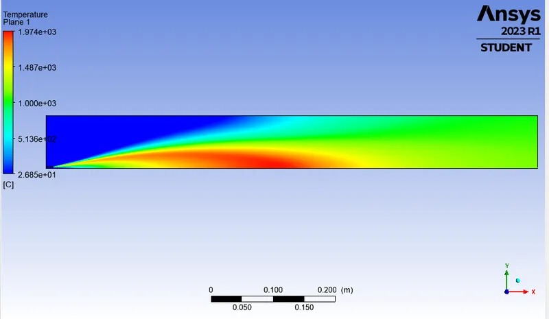
Please refer the below photo for the Temperature plot obtained.

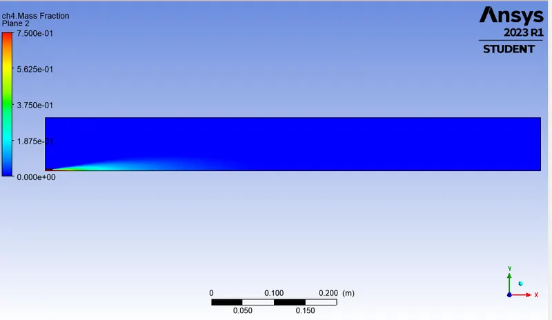
Please refer the below photo for the CH4 Mass fraction plot obtained.

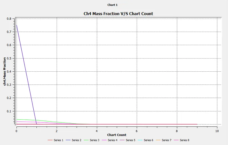
Please refer the below photo for the CH4 Mass fraction Chart obtained.

Please refer the below photo for the CO2 Mass fraction plot obtained.

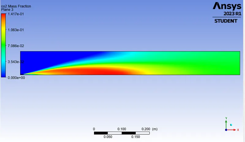
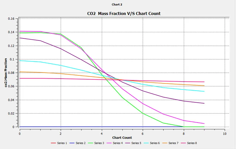
Please refer the below photo for the CO2 Mass fraction Chart obtained.

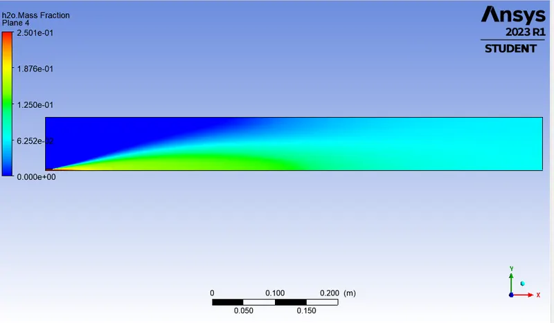
Please refer the below photo for the H20 Mass fraction plot obtained.

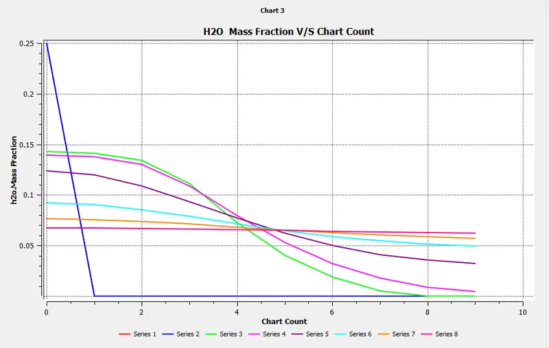
Please refer the below photo for the H20 Mass fraction Chart obtained.

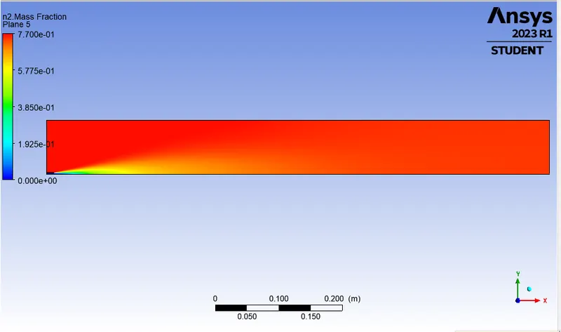
Please refer the below photo for the N2 Mass fraction plot obtained.

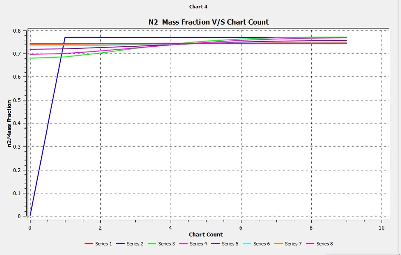
Please refer the below photo for the N2 Mass fraction Chart obtained.

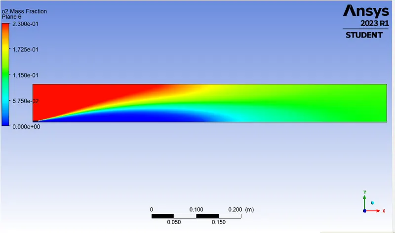
Please refer the below photo for the O2 Mass fraction plot obtained.

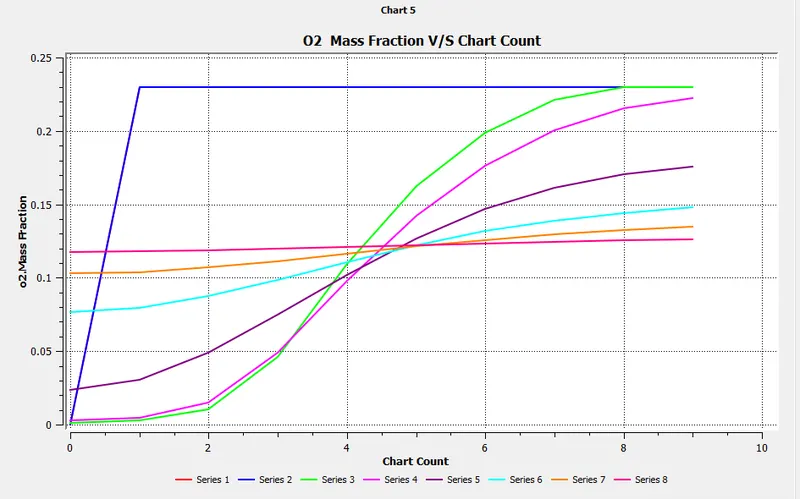
Please refer the below photo for the O2 Mass fraction Chart obtained.

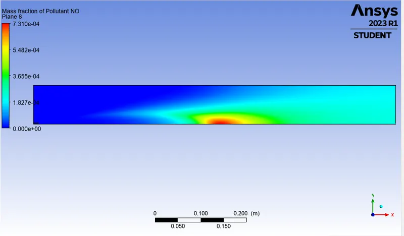
Please refer the below photo for the NO Mass fraction of pollutent plot obtained.

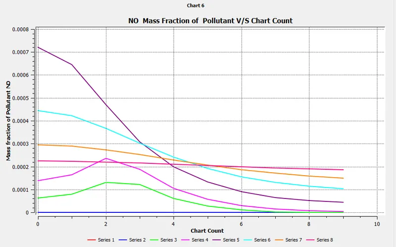
Please refer the below photo for the NO Mass fraction of pollutent Chart obtained.

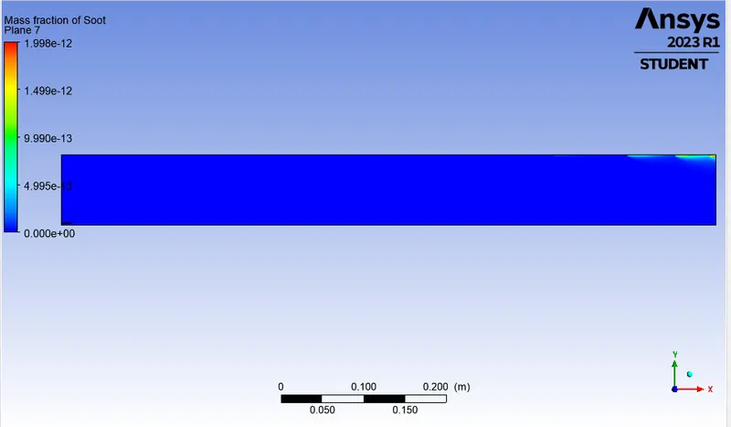
Please refer the below photo for the Mass fraction of Soot plot obtained.

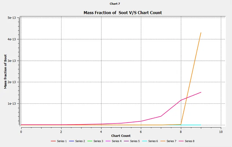
Please refer the below photo for the Mass fraction of Soot Chart obtained.

Please refer the below photo for the results obtained.

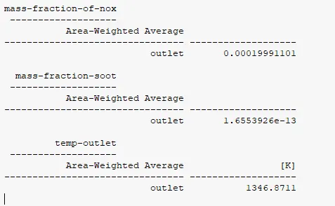
Case 7 : 70% Methane and 30% Water

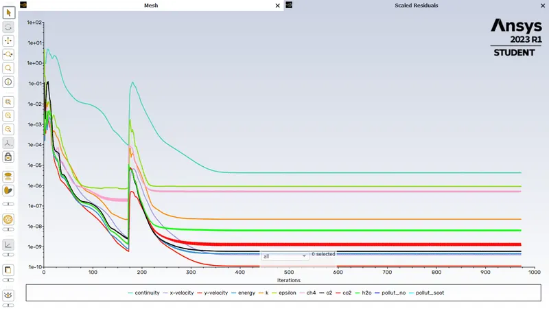
Please refer the below photo for the Residuals obtained.

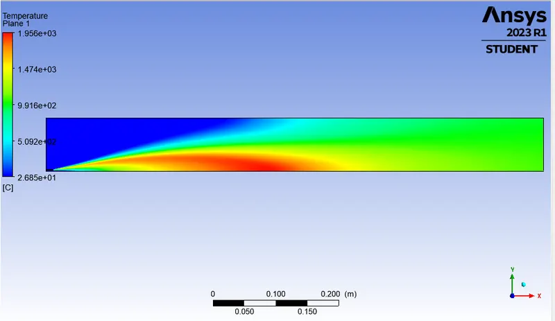
Please refer the below photo for the Temperature plot obtained.

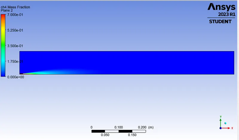
Please refer the below photo for the CH4 Mass fraction plot obtained.

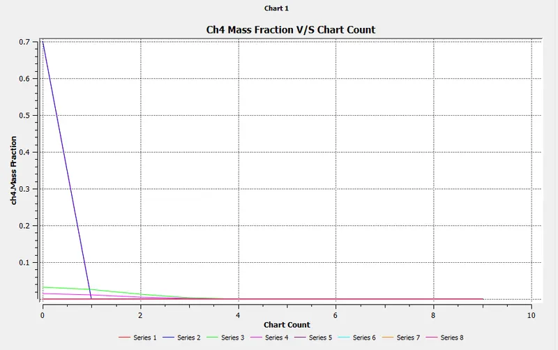
Please refer the below photo for the CH4 Mass fraction Chart obtained.

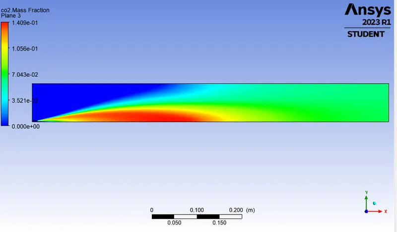
Please refer the below photo for the CO2 Mass fraction plot obtained.

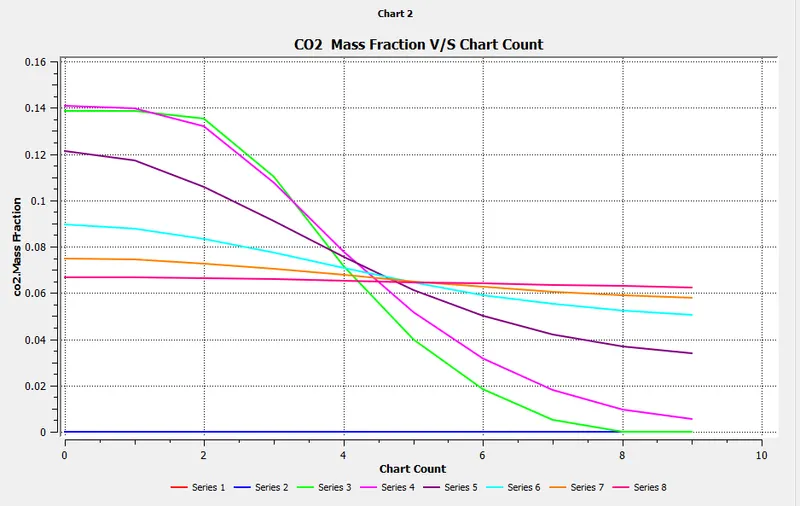
Please refer the below photo for the CO2 Mass fraction Chart obtained.

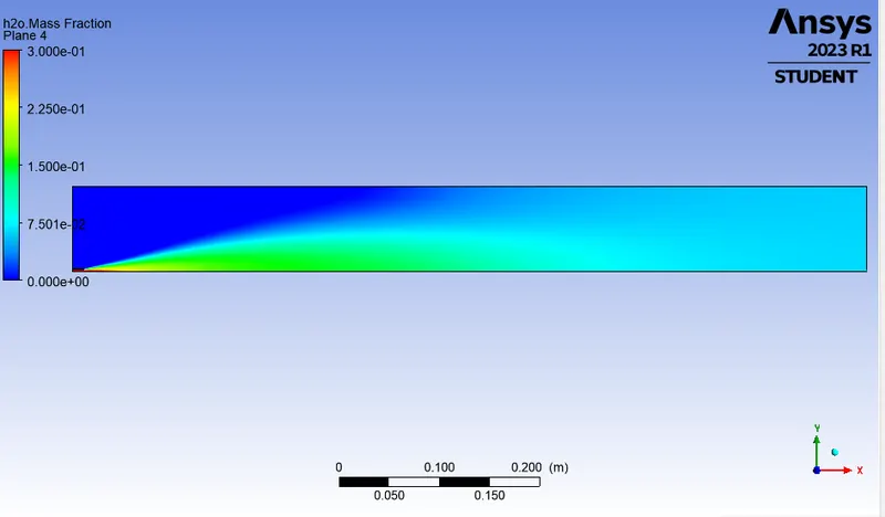
Please refer the below photo for the H20 Mass fraction plot obtained.

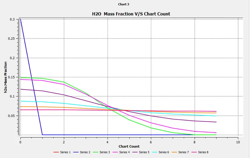
Please refer the below photo for the H20 Mass fraction Chart obtained.

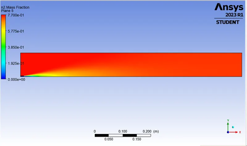
Please refer the below photo for the N2 Mass fraction plot obtained.

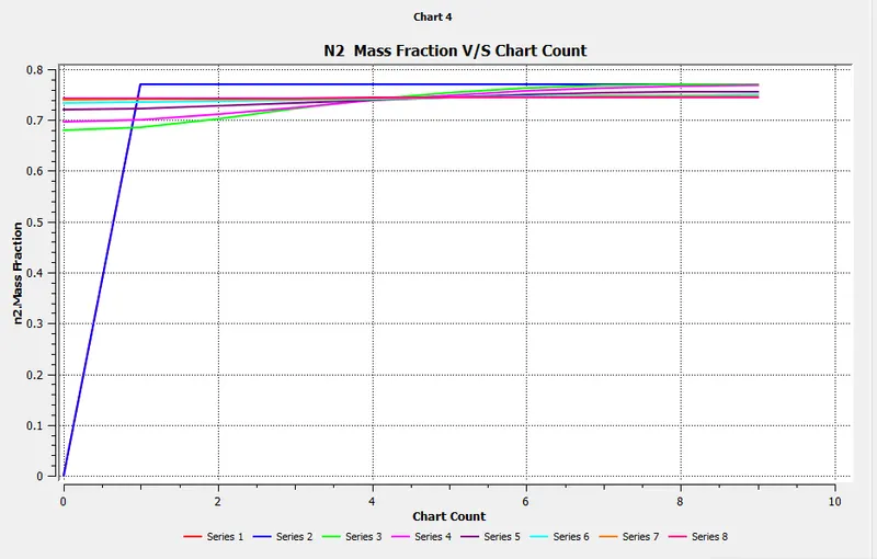
Please refer the below photo for the N2 Mass fraction Chart obtained.

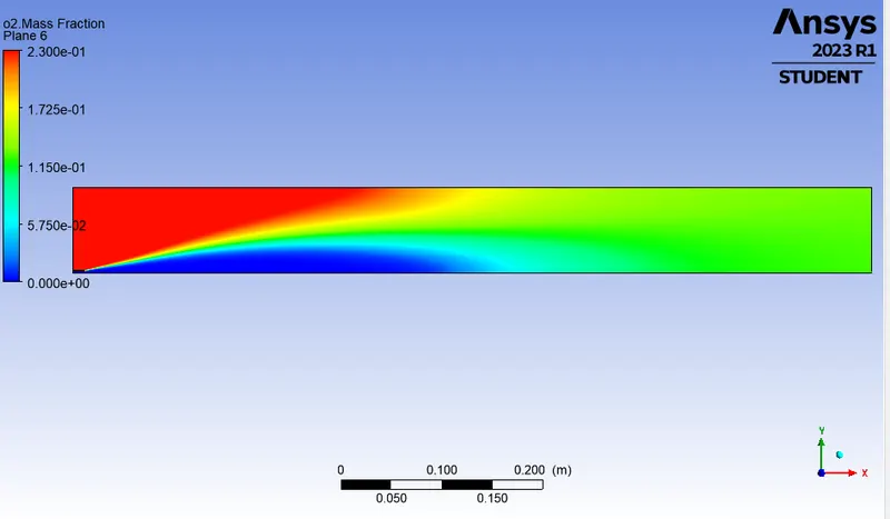
Please refer the below photo for the O2 Mass fraction plot obtained.

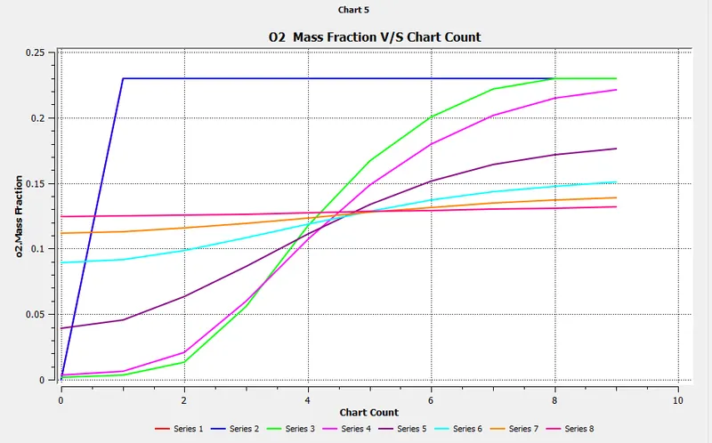
Please refer the below photo for the O2 Mass fraction Chart obtained.

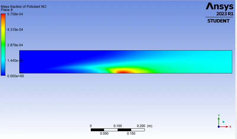
Please refer the below photo for the NO Mass fraction of pollutent plot obtained.

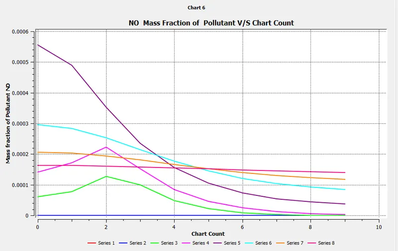
Please refer the below photo for the NO Mass fraction of pollutent Chart obtained.

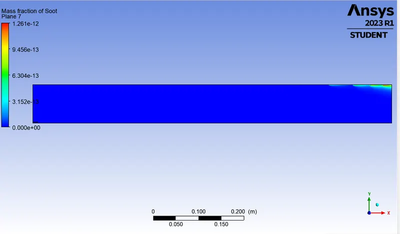
Please refer the below photo for the Mass fraction of Soot plot obtained.

Please refer the below photo for the Mass fraction of Soot Chart obtained.

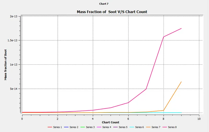
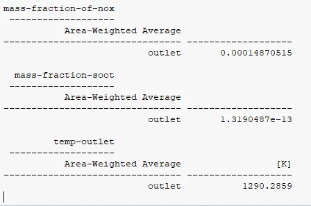
Please refer the below photo for the results obtained.

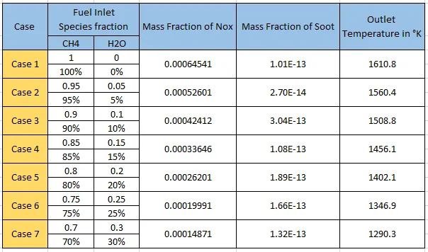
Please refer the below table for consolidated results obtained.

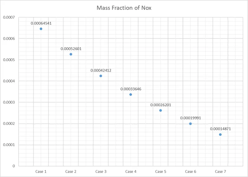
Please refer the below graph of Cases V/S Mass fraction of NOx obtained.

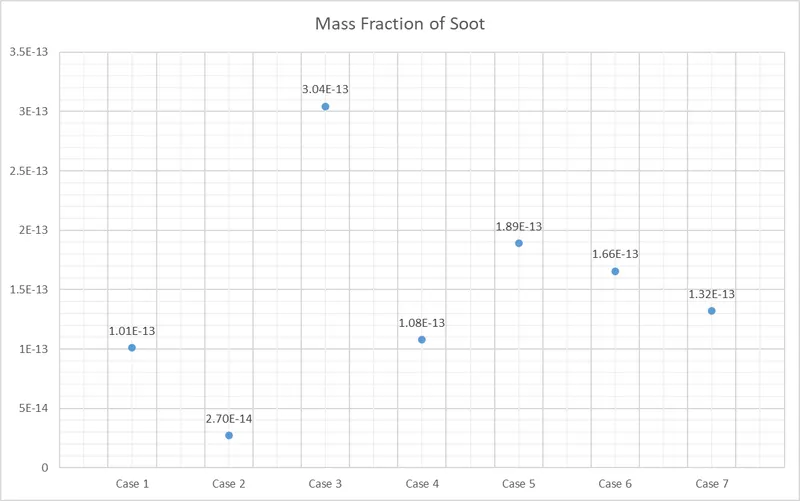
Please refer the below graph of Cases V/S Mass fraction of Soot obtained.

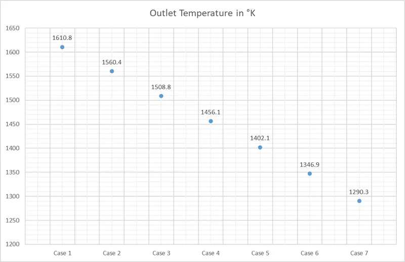
Please refer the below graph of Cases V/S Outlet Temperature obtained.

Please refer the below table for the Parameter table obtained.

Observations and Conclusion:

• After all the work done, the results show pretty interesting results. It is clear that the addition of water have a significant effect on the NOx formation. Independently of the contact mode, as more water is added to the system, less NOx are formed.
• Highest temperature is achieved in the proximity of the Inlet.
• The addition of water has a direct effect in the temperature profile of the system. It reduce the peak temperature and also the average temperature of the system. The temperature reduces from case 1 to case 7 i.e 1610.8 °K to 1290.3 °K.
• Also the Mass fraction of pollutent NOx reduces from case 1 to case 7 i.e 0.00064541 to 0.00014871.
• Since soot value decreases with dilution we can say there is less wastage of fuel, i.e. complete combustion occurs.
• In this project, the mass fraction of pollutants from NOx emission and soot formation is predicted with the help of physical and mathematical models incorparated in the CFD software ANSYS fluent. The results obtained from the simulation shows that the addition of water into the fuel not only decreases the temperature of the combustor but also helps in reducing the mass fraction of pollutants like NOx and soot.