Week 5 - Rayleigh Taylor Instability

AIM: Perform the Rayleigh Taylor instability simulation for heavy and light density fluids at top and bottom respectively by CFD Ansys fluient.

OBJECTIVE:

1. Practical CFD models that have been based on the mathematical analysis of Rayleigh Taylor waves? explain how these mathematical models have been adapted for CFD calculations.
2. Perform the Rayleigh Taylor instability simulation for 2 different mesh sizes with the base mesh being 0.5 mm. Compare the results by showing the animations( Attach them from your google drive). Observe the differences in the animation and explain the effect of mesh size on simulation. Also, explain why a steady-state approach might not be suitable for these types of simulation.[ Choose Air and Water for this simulation]
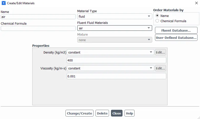
3. Run one more simulation with water and user-defined material(density = 400 kg/m³, viscosity = 0.001 kg/m-s) for refined mesh.
4. Define the Atwood Number. Find out the Atwood number for both the cases and explain how the variation in Atwood number in the above two cases affects the behavior of the instability.

Theory:

Instability:

In dynamical system instability means that some of the outputs or internal states increase with time, without bounds.

Example: Atmospheric instability is a major component of all weather system on Earth.

Fluid instabilities:

Fluid instabilities occur in liquids, gases and plasma, and are often characterized by the shape that form; they are studied in fluid dynamics and magnetohydrodynamics. Fluid instabilities include the following applications

Rayleigh–Taylor instability:

The Rayleigh–Taylor instability, or RT instability is an instability of an interface between two fluids of different densities which occurs when the lighter fluid is pushing the heavier fluid.There are situations where a heavy liquid layer is placed over a lighter fluid layer. This situation has engineering implications in several industries. For example in die casting, liquid metal is injected in a cavity filled with air. In poor designs or other situations, some air is not evacuated and stay in small cavity on the edges of the shape to be casted. Thus, it can create a situation where the liquid metal is above the air but cannot penetrate into the cavity because of instability. y. This instability deals with a dense, heavy fluid that is being placed above a lighter fluid in a gravity field perpendicular to interface. Example for such systems are dense water over oil (liquid–liquid), or water over air(gas–liquid). It can occur under gravity and, equivalently, under an acceleration of the fluid system in the direction toward the denser fluid. A simple example may illustrate typical evolution times for the overturn of ordinary liquids under the effect of the earth's gravity. Assuming an acceleration a = 9.8 m/s2 and a perturbation wavelength A= 1 cm, the classical e-folding time r = Square root of (A/2pai a) of the free-surface RT instability would be 0.013 s. Even if an unstable equilibrium would be established, the instability evolution would be too fast for direct observation.

Supposed that a liquid density is arbitrary function of the height. This distortion can be as a result of heavy fluid above the lighter liquid. The surface tension is the opposite mechanism that will returns the liquid to its original place. This analysis is referred to the case of infinite or very large surface. The simplified case is the two different uniform densities. For example a heavy fluid density,ρH above lower fluid with lower density,ρL. For perfectly straight interface, the heavy fluid will stay above the lighter fluid. If the surface will be disturbed, some of heavy liquid moves down. This disturbance can grow or returned to its original situation. This condition is determined by competing forces, the surface density, and the buoyancy forces. The fluid above the depression is in equilibrium with the sounding pressure since the material is extending to infinity. Thus, the force that acting to get the above fluid down is the buoyancy force of the fluid in the depression.

The depression is returned to its original position if the surface forces are large enough. In that case, this situation is considered to be stable. On the other hand, if the surface forces (surface tension) are not sufficient, the situation is unstable and the heavy liquid enters into the liquid fluid zone and vice versa. As usual there is the neutral stable when the forces are equal. Any continues function can be expanded in series of cosines. Thus, example of a cosine function will be examined. The conditions that required from this function will be required from all the other functions. The disturbance is of the following equation

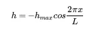
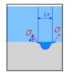
where hmax is the maximum depression and L is the characteristic length of the depression. The depression has different radius as a function of distance from the center of the depression,x . The weakest point is at x=0 because symmetrical reasons the surface tension does not act against the gravity as shown in the below figure.

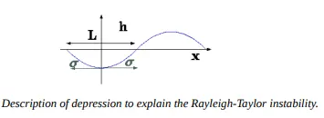
The pressure difference or the pressure jump is due to the surface tension at this point X must be

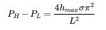-------1

Where PH is the pressure at heavy fluid

PL is the pressure at light fluid

hmax is the maximum depression.

L is the characteristic length of the depression.

`σ` is the surface tension at this point X

The pressure difference due to the gravity at the edge of the disturbance is then

----------2

Where PH is the pressure at heavy fluid

PL is the pressure at light fluid

hmax is the maximum depression.

ρL is the density of light fluid

ρH is the density of heavy fluid

g is the gravitational force i.e 9.81 m/s2.

By comparing the equation 1 and 2 we get

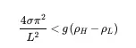
It should be noted that hmax is irrelevant for this analysis as it is canceled. The point where the situation is neutral stable will be

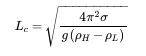
If all the heavy liquid "atempts" to move straight down, the lighter liquid will "prevent" it. The lighter liquid needs to move up at the same time but in a different place. The heavier liquid needs to move in one side and the lighter liquid in another location. In this process the heavier liquid "enter" the lighter liquid in one point and creates a depression as shown in the below figure.

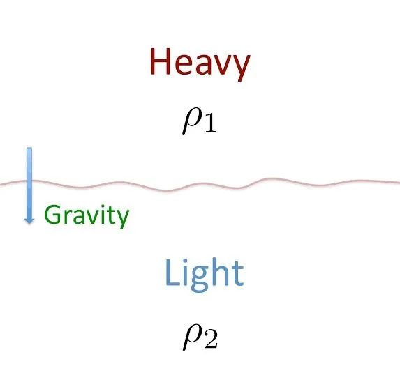
Please refer the below animation for the Rayleigh–Taylor instability

Richtmyer–Meshkov instability:

The Richtmyer–Meshkov instability (RMI) occurs when two fluids of different density are impulsively accelerated. Normally this is by the passage of a shock waves. The development of the instability begins with small amplitude perturbations which initially grow linearly with time. This is followed by a nonlinear regime with bubbles appearing in the case of a light fluid penetrating a heavy fluid, and with spikes appearing in the case of a heavy fluid penetrating a light fluid.

Please refer the below animation for the Richtmyer–Meshkov instability.

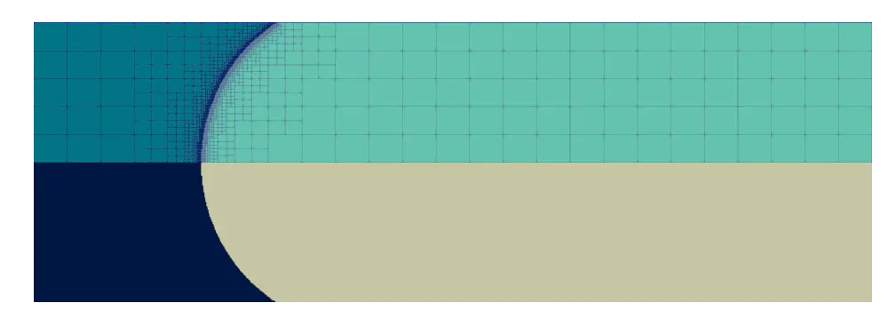
This very complex flow shows two major phenomena due to a high-speed bubble of water impacting a wall (on the left): A right-moving shock wave is created. One can then observe the typical interaction of a bubble that contains heavy fluid (water) in a lighter fluid (air) with Richtmyer-Meshkov instabilities. The impact on the wall also creates left-moving expansion waves leading to the appearance of cavitation pockets due to the decreasing pressure.

Kelvin–Helmholtz instability:

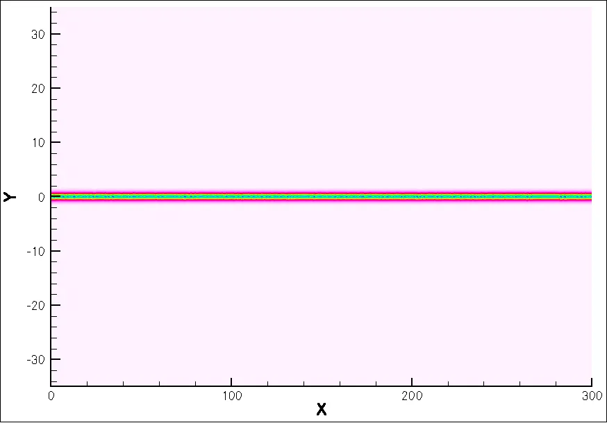
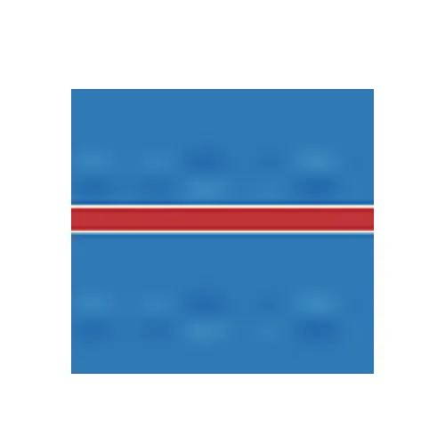
The Kelvin–Helmholtz instability is a fluid instability that occurs when there is velocity sharing in a single continuous fluid or a velocity difference across the interface between two fluids. Kelvin-Helmholtz instabilities are visible in the atmosphere of planets and moons, such as in cloud formation on earth or the Read Spot on Jupitor, and the atmosphere of the sun and other stars.

Please refer the below animation for the Kelvin–Helmholtz instability.

Plateau–Rayleigh instability:

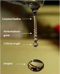
The Plateau–Rayleigh instability, often just called the Rayleigh instability, explains why and how a falling stream of fluid breaks up into smaller packets with the same volume but less surface area. It is related to the Rayleigh–Taylor instability and is part of a greater branch of fluid dynamics concerned with fluid thread backup. This fluid instability is exploited in the design of a particular type of ink jet technology whereby a jet of liquid is perturbed into a steady stream of droplets.

Please refer the below photo and animation of the Plateau–Rayleigh instability for the water droplets from the tap.

Saffman–Taylor instability:

Saffman-Taylor instability is what we call the instability that arises when you displace a more vicious fluid by a less viscous fluid. Experimentally we injected water into glycerol and air into glycerol in order to see the effects of Saffman-Taylor instability on the interface between the two fluids which resulted in interesting fingering patters as seen below:

Multiphase:

Multiphase flow is a simultaneous flow of materials with different states or phases

It is a flow of materials with different chemical properties but in the same state or phase

Types of phases in Multiphase

1. Separated phase:It is defined as the one or more immiscible fluid in a continuous phase is separated by an interface.

2. Mixed phase:It is defined as the phase in which one or more fluids mixed together. It contains both separated and Dispersed phase.

3. Dispersed phase:It is defined as the phase in which finite number of phases are separated in the continuous phase.

VOF (Volume of fraction)model:

The VOF model can model two or more immiscible fluids by solving a single set of momentum equations and tracking the volume fraction of each of the fluids throughout the domain. Typical applications include the prediction of jet breakup, the motion of large bubbles in a liquid, the motion of liquid after a dam break, and the steady or transient tracking of any liquid-gas interface.

The VOF formulation in ANSYS FLUENT is generally used to compute a time-dependent solution, but for problems in which you are concerned only with a steady-state solution, it is possible to perform a steady-state calculation. A steady-state VOF calculation is sensible only when your solution is independent of the initial conditions and there are distinct inflow boundaries for the individual phases. For example, since the shape of the free surface inside a rotating cup depends on the initial level of the fluid, such a problem must be solved using the time-dependent formulation. On the other hand, the flow of water in a channel with a region of air on top and a separate air inlet can be solved with the steady-state formulation.

For example consider α1=Phase 1, α2=Phase 2

then VOF should be α1+α2=1

Courant Number:

The Courant number in one-dimension is defined as C ≡ u∆t /∆x where u is the characteristic wave speed of the system, ∆t is the time-step of the numerical model, and ∆x is the spacing of the grid in the numerical model.

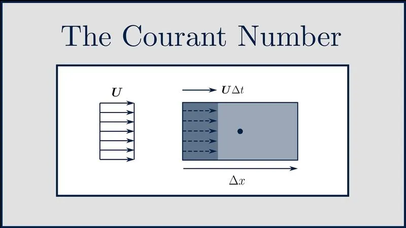
It is a non-dimensional number that tells how fast information travels through our descretization domine.

The Courant number can be used in Computational Fluid Dynamics (CFD) simulations to evaluate the time step requirements of a transient simulation for a given mesh size and flow velocity and is linked to the Courant–Friedrichs–Lewy (CFL) stability condition of numerical schemes.

The Courant number plays an important role when running a transient CFD simulation, where we are interested in the variations of the flow field in time as well as in space. The physical time is discretised using a time step and the choice of time step has two main implications: one is related to the stability of the time discretisation scheme; the other is related to the physical meaning of the time step. CFL value less than or equal to 1 will give good simulation.

Explicit Scheme:

It offers time accurate data, but the time steps size has to be taken ensuring that the Courant number satisfied

Implicit Scheme:

It will offer the speed of the steady state but need a time varying solution. It is unconditionally stable (time step size is not a constraint).

Why Transient State solver time used in this problem?

In this RT instability due to sudden collapse of horizantal plane between denser and lighter fluid, shock waves are generated and due to this reason bubble and spike formation takes place. Simulation involves capturing instabilities that are changing in an unpredictable manner as a function of time, thus the transient approach is preferred over the steady state approach.

Atwood number:

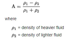
The Atwood number is a dimensionless number in fluid dynamics used in the study of hydrodynamic instabilities in density-stratified flows. The Atwood number equals the ratio of the difference in mass densities to their sum.

It is a dimensionless density ratio defined as below

Atwood number Significance:

Higher the atwood number the instebilities are sudden and reach

Lower the atwood number instabilities take time and reach steady state slowly

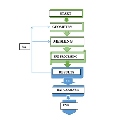
Please refer the below chart for the CFD flow analysis for the simulation of Rayleigh Taylor instability to heavy and light density fluids at top and bottom respectively.

Geometry Setup:

Following steps were followed in the Geometry Setup.

1) Open the Space domine

2) Use the rectangle tool & then creat a rectangle 20x20 from the origin. Then use the pull comand to convert the rectangle to surface for water and at the top. Then creat a new component and again creat a another surface at the bottom to the previous surface created air/user define material at the bottom as shown in the below

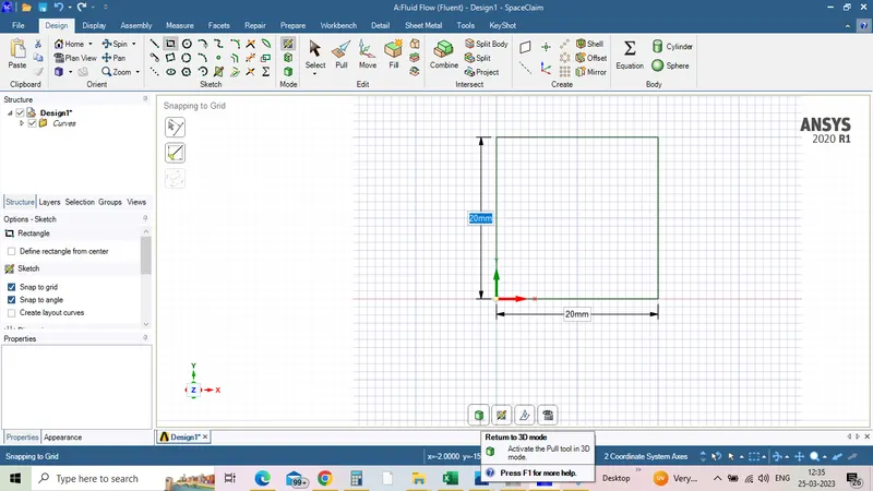
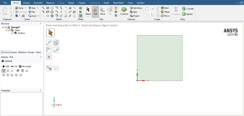
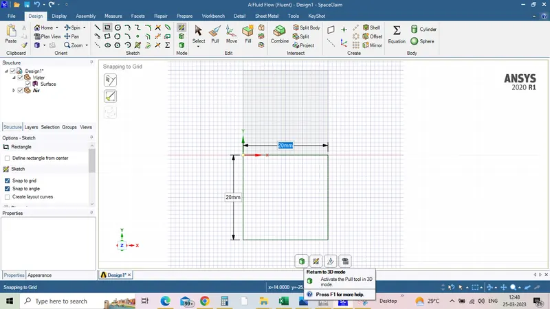
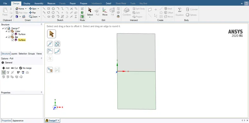
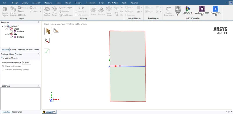
3) Then use the share tool to share the interface between the surface as shown below.

Meshing:

Mesh independent study has to be done for the 3 different cases for water and air phase and 1 case for the water and user defined phase.

Case 1:

For the case 1 the mesh element size is 0.5 mm Nodes no 3321 is and Element no 3200 as shown below.

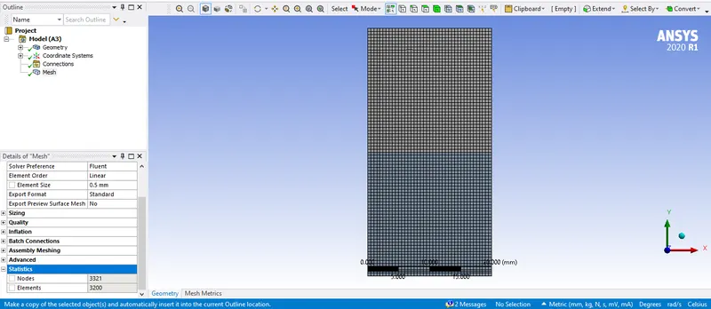
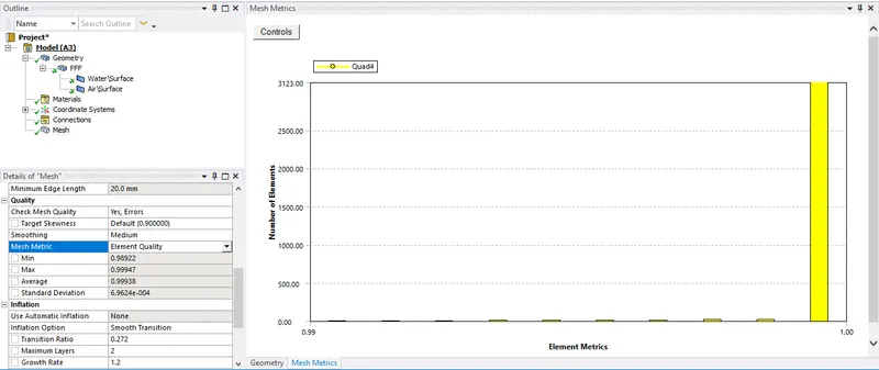
The average elemental quality is 0.99938 please refer the below photo for it

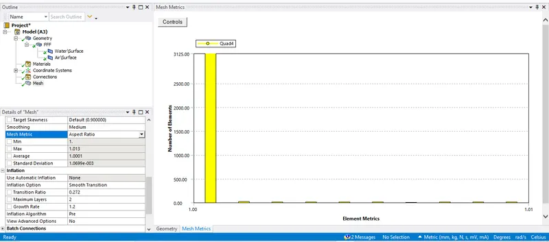
The average Aspect ratio is 1.0001 please refer the below photo for it

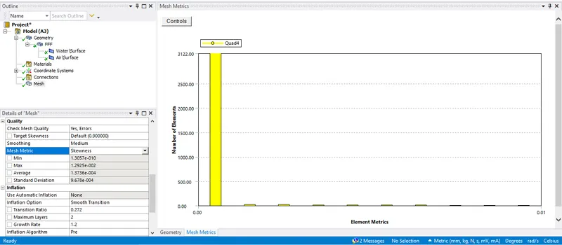
The average Skewness is 1.3736e-4 please refer the below photo for it

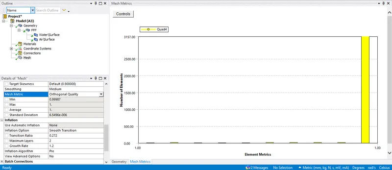
The average Orthogonality is 1 please refer the below photo for it

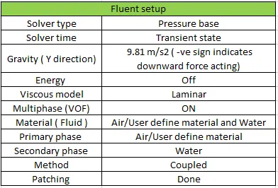
Please refer the below table for the fluient set up applied.

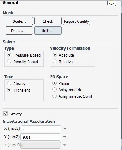
Please refer the below photo for the solver type , solver time and Gravity applied.

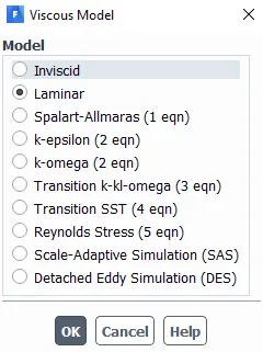
Please refer the below photo for the Viscous model applied.

Please refer the below photo for the Material applied.

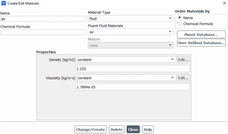
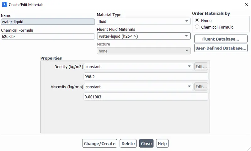
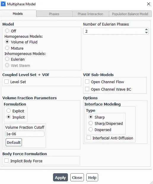
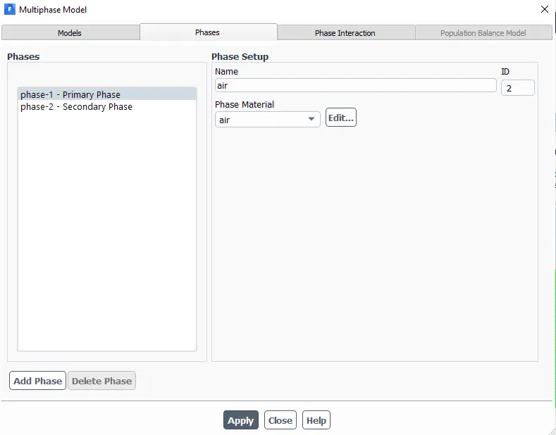
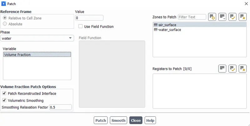
Please refer the below photo for the Multiphase, VOF and Implicit applied.

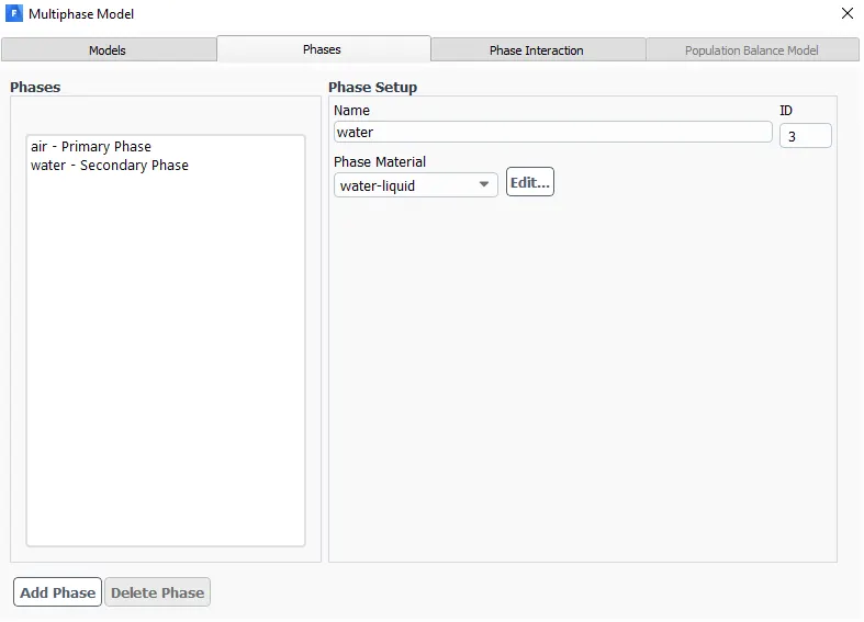
Please refer the below photo for the Hybrid initialization applied.

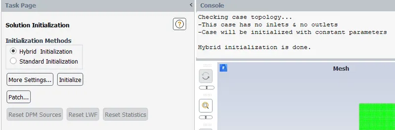
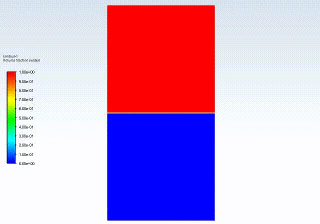
Please refer the below photo for the Contour applied for the phase.

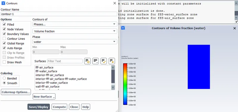
Please refer the below photo for the Patching done for the air and water.

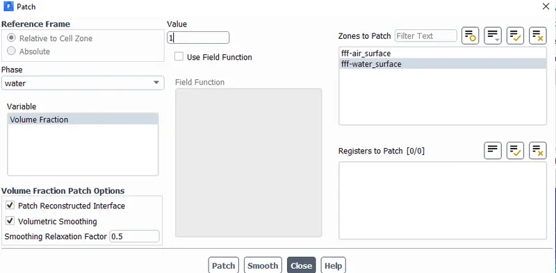
After Patching it look like as below.

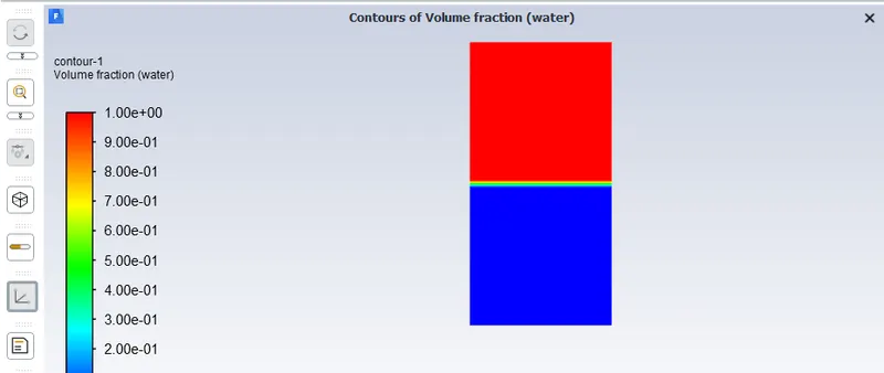
This fluient setup is same for both case 2 and Case 3.

Time steps is given as shown below.

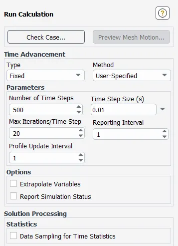
Results:

Please refer the below photo for the Residuals obtain

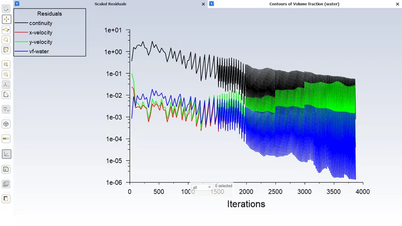
Please refer the below animation obtained at the end.

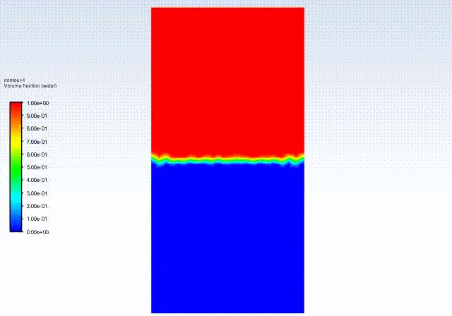
Case 2:

For the case 2 the mesh element size is 0.3 mm Nodes no 9180 is and Element no 8978 as shown below.

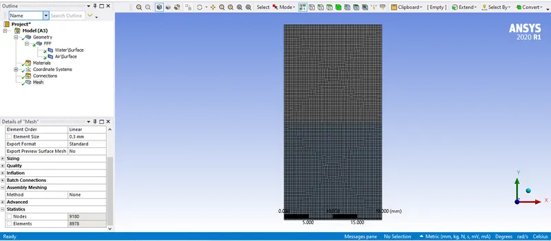
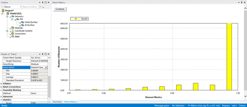
The average elemental quality is 0.99612 please refer the below photo for it

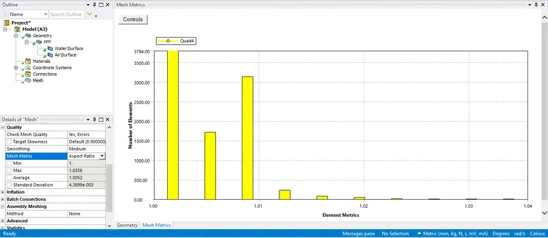
The average Aspect ratio is 1.0052 please refer the below photo for it

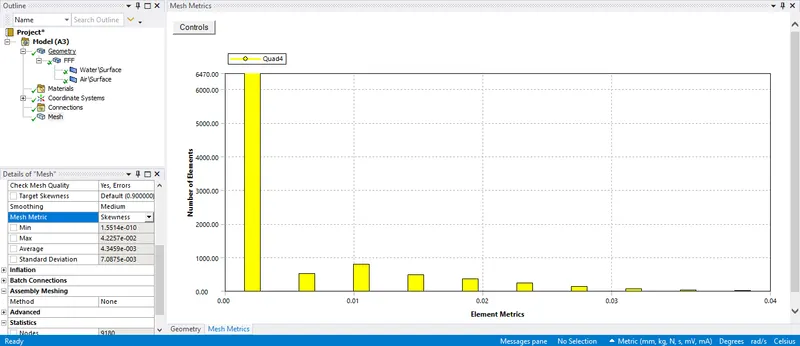
The average Skewness is 4.3459e-3 please refer the below photo for it

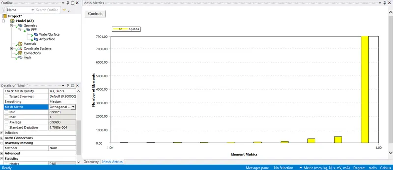
The average Orthogonality is 0.99993 please refer the below photo for it

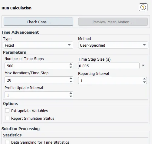
Time steps is given as shown below.

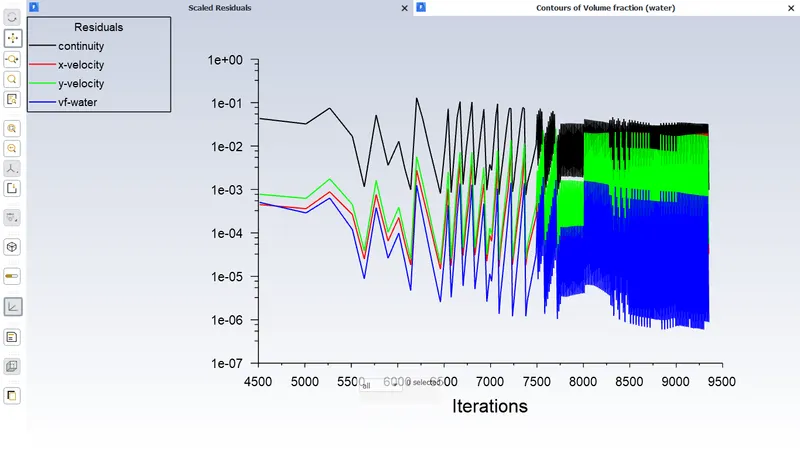
Results:

Please refer the below photo for the Residuals obtain

Please refer the below animation obtained at the end.

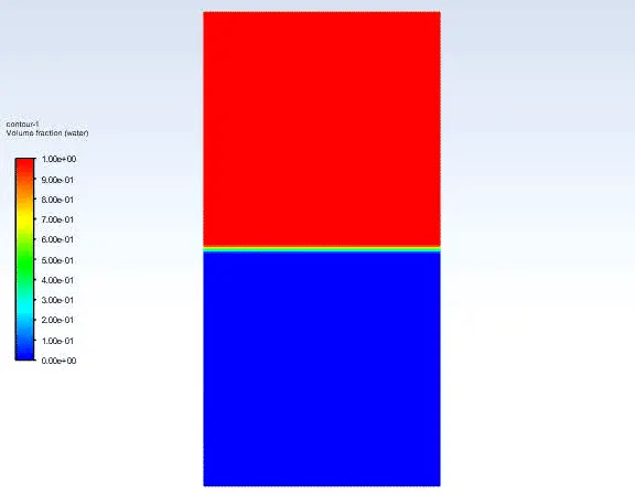
Case 3:

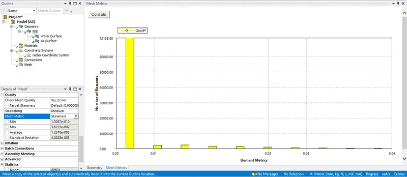
For the case 3 the mesh element size is 0.1 mm Nodes no 80601 is and Element no 80000 as shown below.

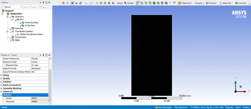
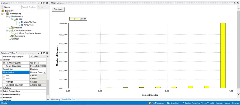
The average elemental quality is 0.99853 please refer the below photo for it

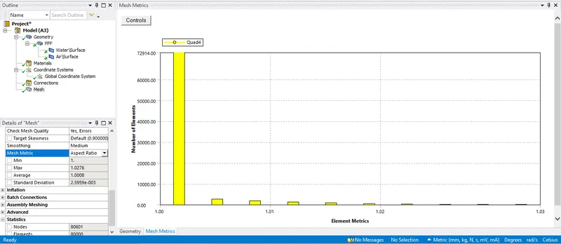
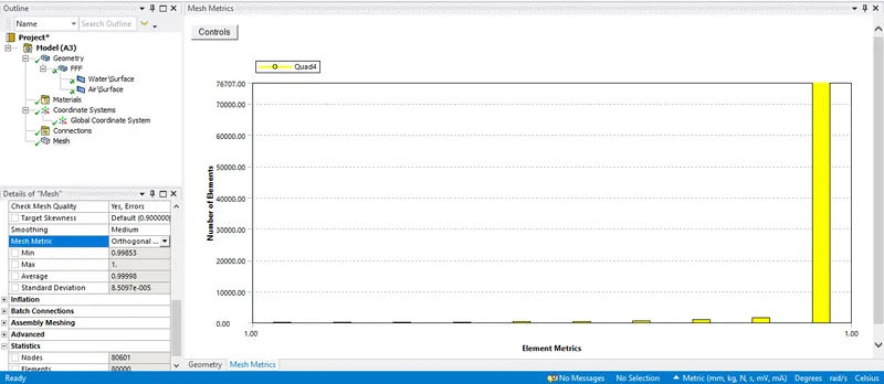
The average Aspect ratio is 1.0008 please refer the below photo for it

The average Skewness is 1.2318e-3 please refer the below photo for it

The average Orthogonality is 0.99998 please refer the below photo for it

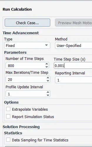
Time steps is given as shown below.

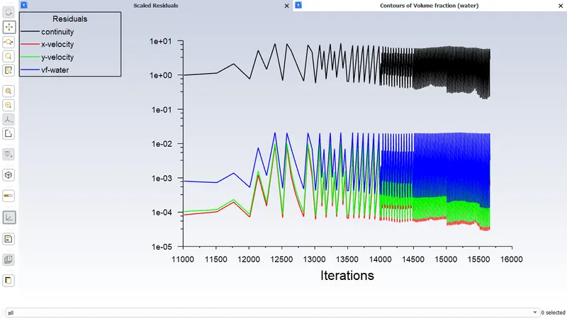
Results:

Please refer the below photo for the Residuals obtain

Please refer the below animation obtained at the end.

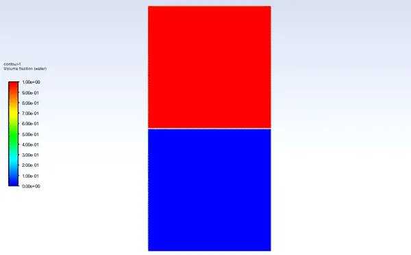
Case 4:

Meshing set up for the case 4 is same as the case 3.

Fluient set up will be same as in case 1 except the User define material as shown below.

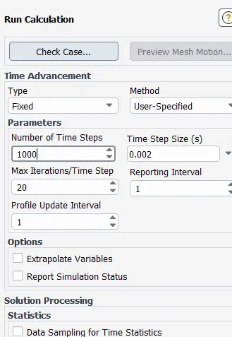
Time steps is given as shown below.

Results:

Please refer the below photo for the Residuals obtain

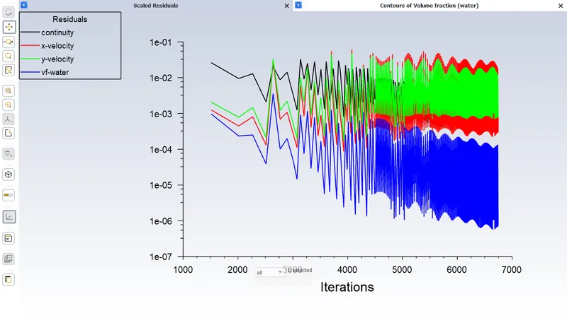
Please refer the below animation obtained at the end. I have recorded for every 10 time steps so it seems to be fast animation.

Atwood Number:

As we discussed previous it is given by

For case 1, case2 and case 3 density of air is 1.225 kg/m3 and density of water is 998.2 kg/m3.

Atwood number=(998.2-1.225)/(998.2+1.225)=996.975/999.425

Atwood number=0.99754

For case 4 density of air/User define material is 400 kg/m3 and density of water is 998.2 kg/m3.

Atwood number=(998.2-400)/(998.2+400)=598.2/1398.2

Atwood number=0.42783

Conclusion:

• As the mesh become finer the mixing will be much more clear and visible also increases computational time.
• Finer mesh shows the formation of bubbles observed.
• For lower atwood number (Case 4)bubble and mushroom head shape is relatively symmetrical, the disturbence are linear for a large time.
• For higher atwood number (Case 1,2 and 3)bubble and mushroom head shape is less symmetrical, also it occurs very rapidly at an acclerating rate which leads to a non-linear growth rate.