Week 1- Mixing Tee
Aim: In this challenge, we have abtain the two versions of the mixing tee. One of them is longer than the other.To set up steady-state simulations to compare the mixing effectiveness when hot inlet temperature is 360C & the Cold inlet is at 190C.
Use the k-epsilon and k-omega SST model for the first case and based on your judgment use the more suitable model for further cases. Giving the reason for choosing a suitable model is compulsory.
- Case 1
- Short mixing tee with a hot inlet velocity of 3m/s.
- Momentum ratio of 2, 4.
- Case 2
- Long mixing tee with a hot inlet velocity of 3m/s.
- Momentum ratio of 2, 4.
Momentum ratio = velocity at cold inlet / velocity at hot inlet
In a table, compare the following values from the 2 cases.
- Cell count
- Average outlet temperature
- Number of iterations for convergence
Objective:
- Velocity and temperature contour plots on the cut planes along and across the pipe.
- Velocity and temperature line plots along and across the length of the pipe.
- Perform Mesh independent study for any one case.
- Discuss the effect of length and momentum ratio on results.
For each simulation, you need to show the convergence plot.
Theory about Mixing tee:
T-junctions are widely used to facilitate the mixture of two fluids at different temperatures and in most cases, different velocity also. Temperature of the mixture at the outlet of the main pipe undoubtedly plays a significant role in all the industries where T-junctions are implemented as their main intention is to get reduced temperature of the fluid. This paper deals with the three main cases which are expected to rather have a significant impact on the outlet temperature viz. short tee, increased velocity ratio and long tee respectively.
A Tee is formed by two pipe sections joined at a right angle to each other. The hot fluid (air) is flowing through the main pipe while the cold fluid (air) enters the main pipe through the branched pipe. There have been traditionally developed empirical design equations to solve the mixing problems but it does not take into account the complexity of turbulent flow in applications like petrochemical products, waste water treatment, blending of oils, etc.
With due respect to all the other industries, nuclear industry is the one where efficiency of the mixing of fluids in the mixing chambers is very critical. There have been much of research regarding the thermal stresses arising in the T-junctions due to the large temperature difference and also due to frequent changes in the same.
A large temperature gradient is created along the length of the pipe due to mixing of fluids near the junction as well as to the downstream of the main pipe.
Mixing tee possess two inlets and one outlet. The momentum ratio for this type of tee is the ratio of velocity of cold fluid to velocity at mixed fluid at outlet.
In this problem we are taken the moment ratio of 2 and 4 for the hot inlet velocity of 3 m/s, so the cold inlet velocity is 6 m/s and 12 m/s respectively.
Mixing of the fluids inside the pipe was simulated using ANSYS Fluent, a general purpose three dimensional CFD package. The turbulence model selected to setup the required case was k-ℇ realizable and k-Ω SST model by RNAS (Reynolds-Averaged Navier-Stokes) method. Though Large Eddy Simulations (LES) and Direct Numerical Simulation(DNS) will give most accurate results in this case as it involves turbulent mixing, but many experiments have agreed to the fact that k-ℇ realizable and k-Ω SST model reasonably agrees with the experimental results. RANS method is much more quicker than LES and DNS method.
When comparing k-ℇ realizable and k-Ω SST model, k-Ω SST model is much more effective than the k-ℇ realizable. The hot and cold outlet temperatures predicted by the standard and SST k-Ω models are also very close to the experimental values thus we are used k-Ω SST model to solve the problem.
Mass flow rate m(hot) and m(cold) is given by the formula `m(hot)=ρ(Density of air)A(hot)V(hot)` and `m(Cold)=ρ(Density of air)A(cold)V(cold)`respectively.
Mass flow rate at the hot inlet m(hot)=1.225*0.0009*3=0.0033075 kg/s
Mass flow rate at the cold inlet for moment ratio 2, m(cold)=1.225*0.0002*6=0.00147 kg/s
Mass flow rate at the cold inlet for moment ratio 4, m m(cold)=1.225*0.0002*12=0.00294 kg/s
The temperature mixture at the outlet is given by the formula `T(Mixture)=(m (hot)*T (hot)+m (cold)*T (cold))/(m (hot)+m (cold))`
T(mixture) for moment ratio 2, T(hot) is 360C and T(Cold) is 190C with the respective mass flow rate as discussed above is given by the following
T(mixture)=0.0033075*36+0.00147*19/(0.0033075+0.00147)=0.147/0.004545=32.3430C----i
T(mixture) for moment ratio 4, T(hot) is 360C and T(Cold) is 190C with the respective mass flow rate as discussed above is given by the following
T(mixture)=0.0033075*36+0.00294*19/(0.0033075+0.00294)=0.17493/0.0062475=280C----ii
Geometry of Short and Long tee models:
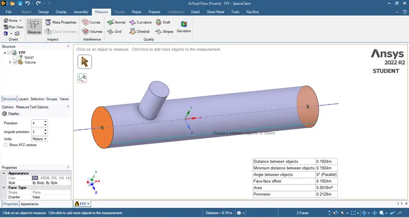
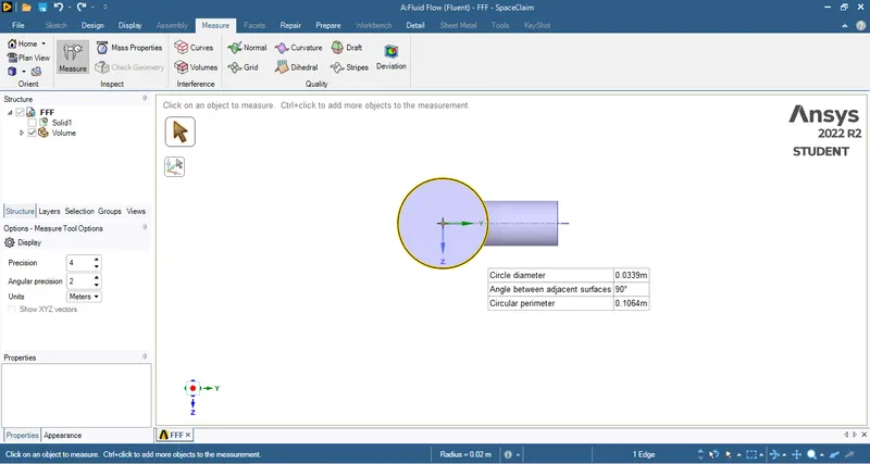
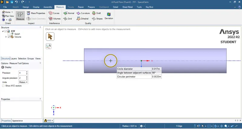
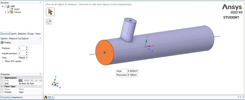
Short tee: Extract the volume from the geometry initialy and start checking the dimensions.The short tee model has the dimension of overall length 0.1924m, hot air inlet diameter of 0.0339m, cold air inlet diameter of 0.017 m and the area of both the hot and cold inlet is 0.0009 m2 and 0.0002 m2 respectively.
Please refer the below photo of geometrical dimensions of the shoet tee model
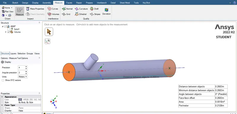
Long tee: In the long tee all the dimensions are same as in the short tee except the overall length i.e 0.2683 m
Please refer the below photo of geometrical dimensions of the long tee model
Meshing of Short and Long tee models:
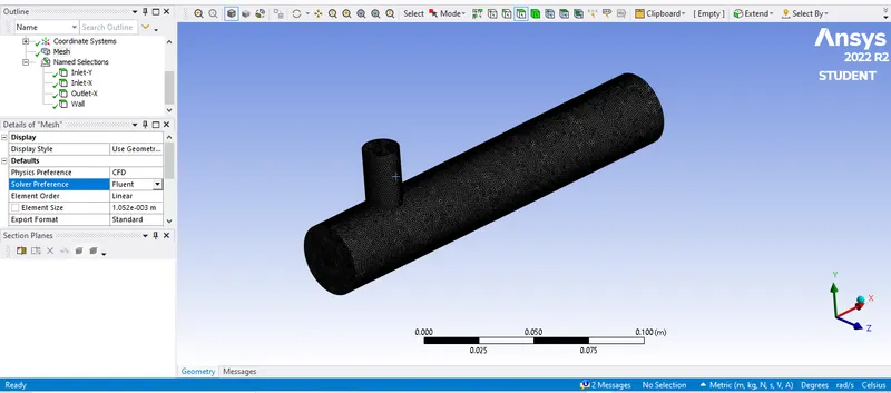
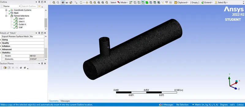
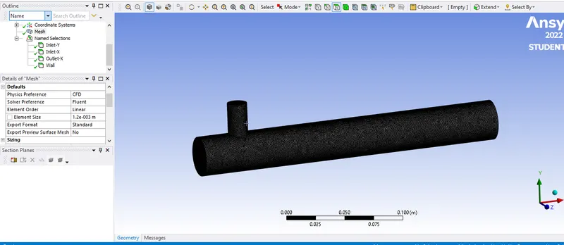
Meshing of short tee model: Tetrahedral elements with size of 0.0001052 m are usedand number of elements and nodes are 510147 and 98153 respectively.
Please refer the below photo of mesh size given and inlet, outlet and wall nomenclature
Please refer the below photo of element and nodes obtained.
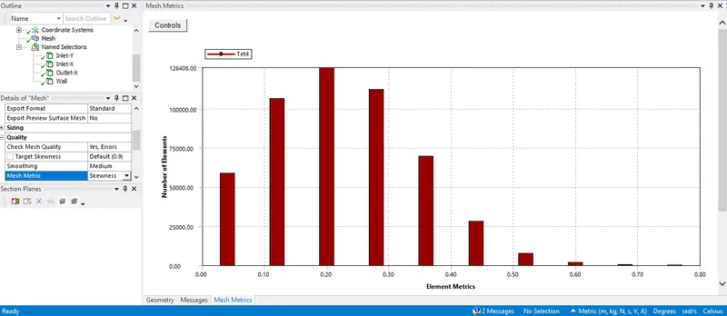
Please refer the below photo for the mesh quality skewness obtained vary between 0-0.8
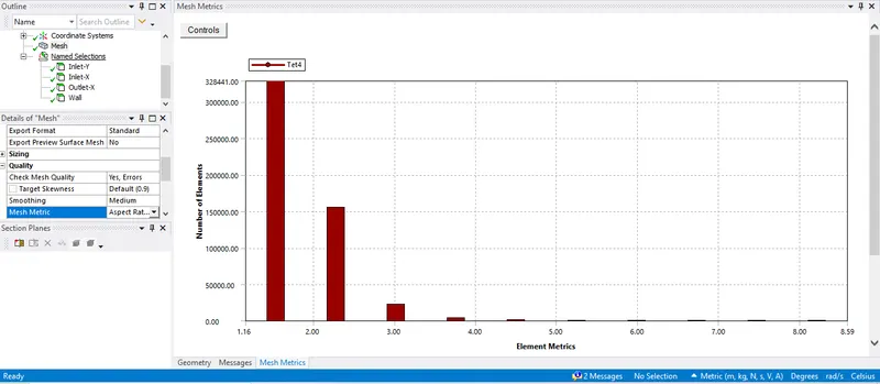
Please refer the below photo for the mesh quality aspect ratio obtained
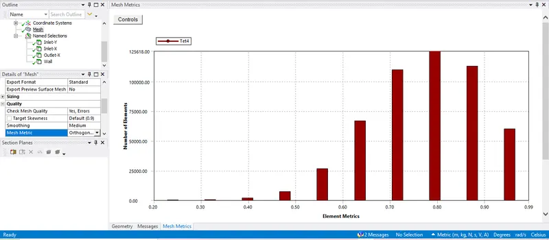
Please refer the below photo for the mesh quality ortogonality obtained
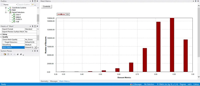
Please refer the below photo for the mesh quality mesh element quality obtained
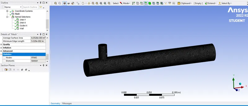
Meshing of Long tee model: Tetrahedral elements with size of 0.00012 m are usedand number of elements and nodes are 504561 and 97642 respectively.
Please refer the below photo of mesh size given and inlet, outlet and wall nomenclature
Please refer the below photo of element and nodes obtained.
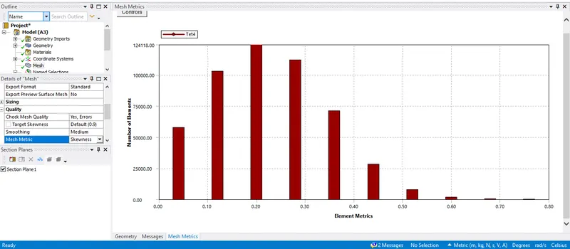
Please refer the below photo for the mesh quality skewness obtained
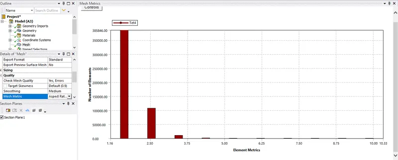
Please refer the below photo for the mesh quality aspect ratio obtained
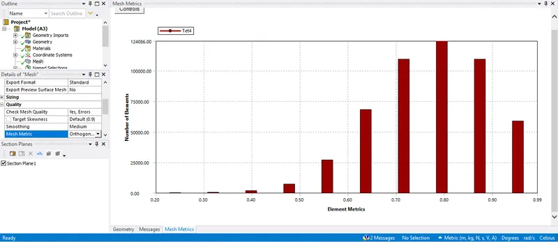
Please refer the below photo for the mesh quality ortogonality obtained
Please refer the below photo for the mesh quality mesh element quality obtained
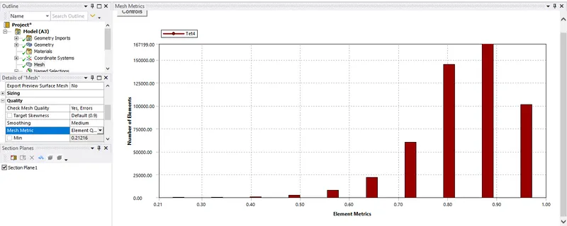
Mesh results:
| Type of Tee | Short Tee |
| Type of mesh method | Triangle |
| Mesh element size | 1.052e-3 m |
| Nodes | 98153 |
| Elements | 510147 |
| Type of Tee | Long Tee |
| Type of mesh method | Triangle |
| Mesh element size | 1.2e-3 m |
| Nodes | 97642 |
| Elements | 504561 |
Setup the Short and Long tee models with different case study:
After meshing we are going to setup the model by double click on double precission, solver process 4, MPI Types intel atlast click on ok.
As there is no change in the density we are using the Solver type as Pressure-Based. Check the mesh quality. Set the units as 0C for temperature. In the model turn on the energy mode and apply the turbulance model and boundry conditions as per the case study. Define the report for the average Area-weighted-Average of temperature and Standard deviation. Hybrid Initialization has to be done and run the calculation by giveng the number of itirations 150.
Case study 1:
Parameters for the case study 1 is in the below table.
| Type of Tee | Short Tee |
| Moment ratio | 2 |
| Hot air velocity and Temperature | 3 m/s, 360C |
| Cold air velocity and Temperature | 6 m/s, 190C |
| Total elements or cell count | 510147 |
| Turbulance model | k-ℇ realizable |
| Theoritical temperature mixture as per calculated |
30.7690C |
For the above boundry condition following results are obtained.
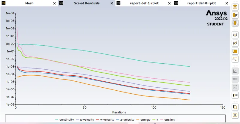
i) Residuals plot
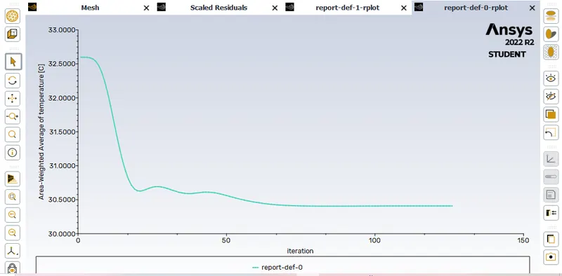
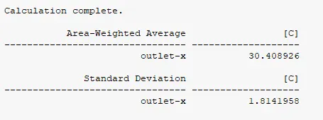
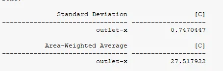
ii) Area-weighted-Average of temperature
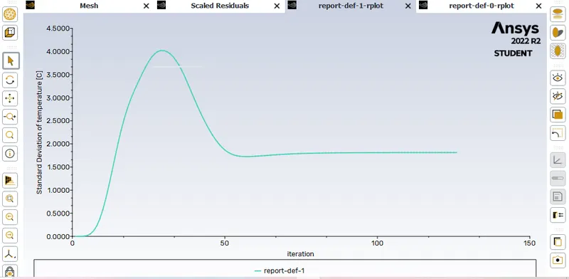
iii) Standard deviation
iv) Result
Post processor results
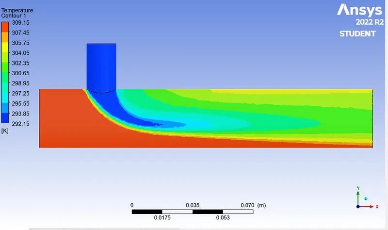
i) Temperature contours plot along the length of the pipe
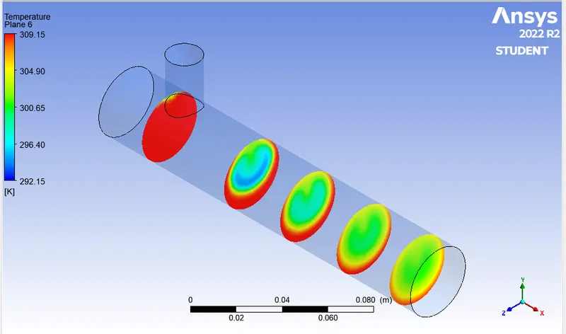
ii) Temperature contours plot across the length of the pipe
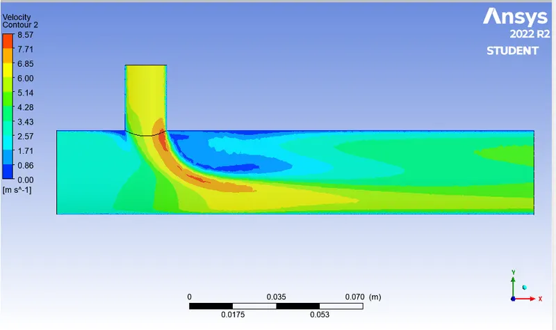
iii) Velocity contours plot along the length of the pipe
iv) Velocity contours plot across the length of the pipe
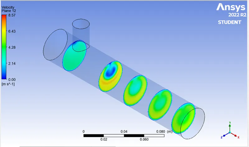
v) Temperature Line plot along the length of the pipe
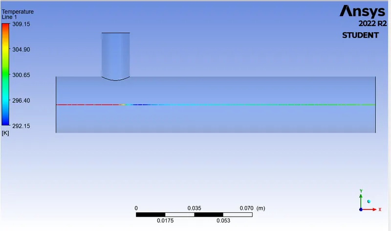
vi) Temperature Line plot across the length of the pipe
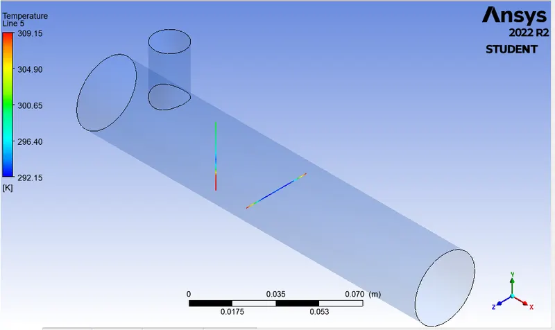
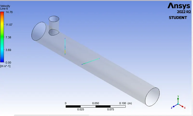
vii)Velocity Line plot along the length of the pipe
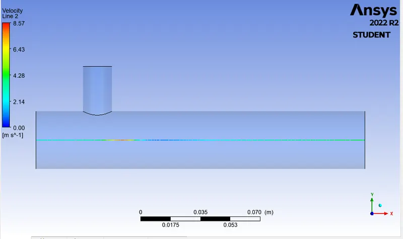
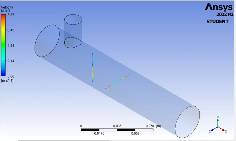
viii) Velocity Line plot across the length of the pipe
Case study 2:
Parameters for the case study 2 is in the below table.
| Type of Tee | Short Tee |
| Moment ratio | 2 |
| Hot air velocity and Temperature | 3 m/s, 360C |
| Cold air velocity and Temperature | 6 m/s, 190C |
| Total elements or cell count | 510147 |
| Turbulance model | k-Ω SST |
| Theoritical temperature mixture as per calculated |
30.7690C |
For the above boundry condition following results are obtained.
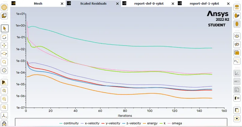
i) Residuals plot
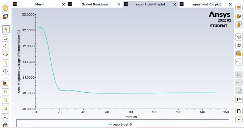
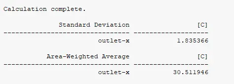
ii) Area-weighted-Average of temperature
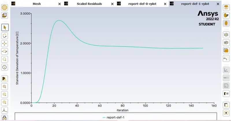
iii) Standard deviation
iv) Result
Post processor results
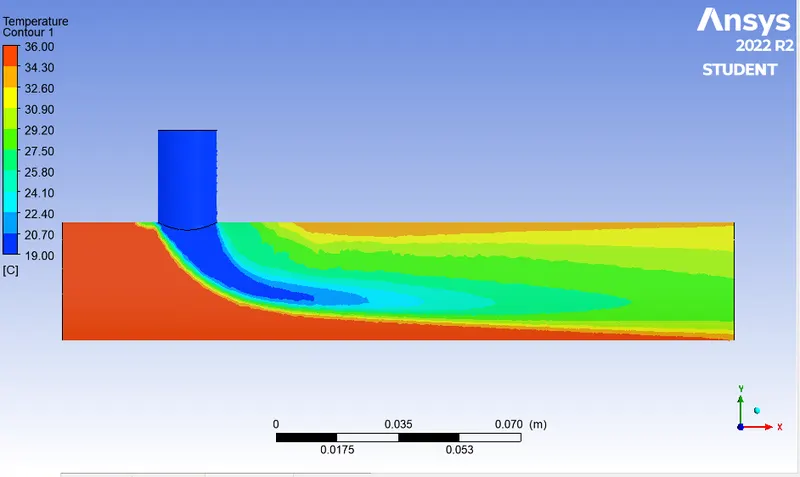
i) Temperature contours plot along the length of the pipe
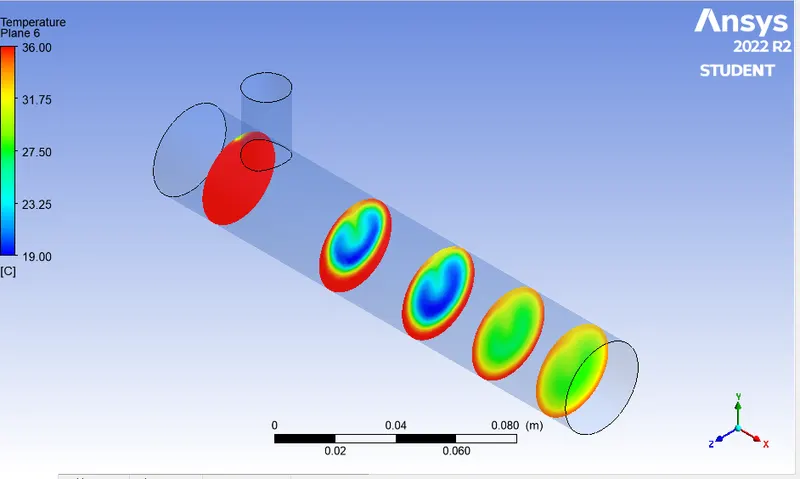
ii) Temperature contours plot across the length of the pipe
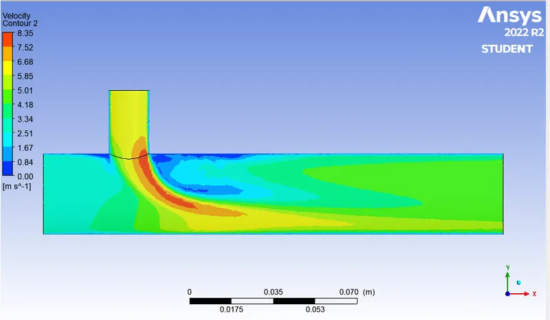
iii) Velocity contours plot along the length of the pipe
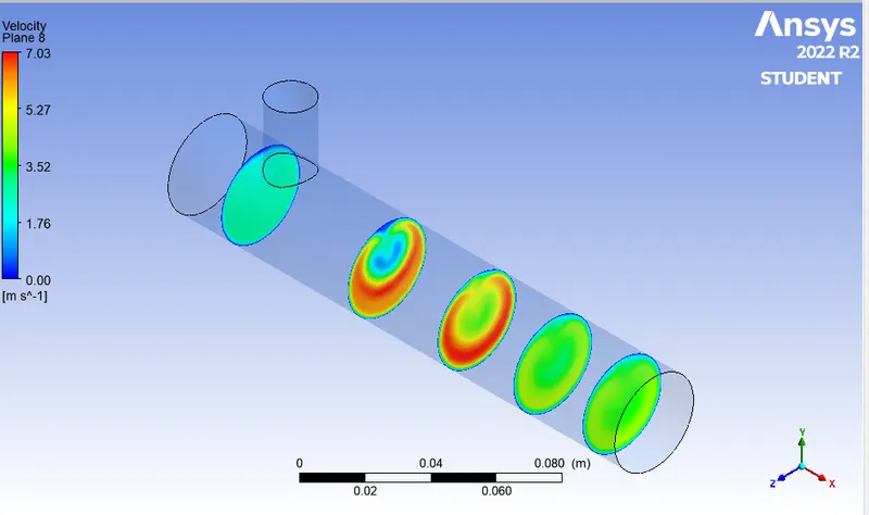
iv) Velocity contours plot across the length of the pipe
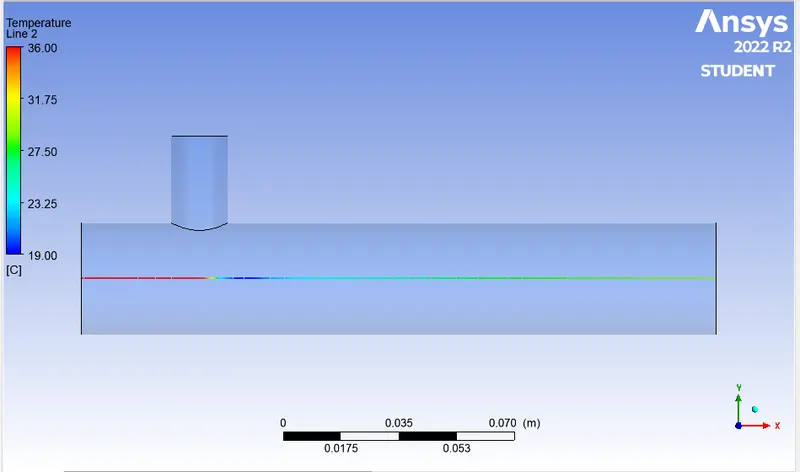
v) Temperature line plot along the length of the pipe
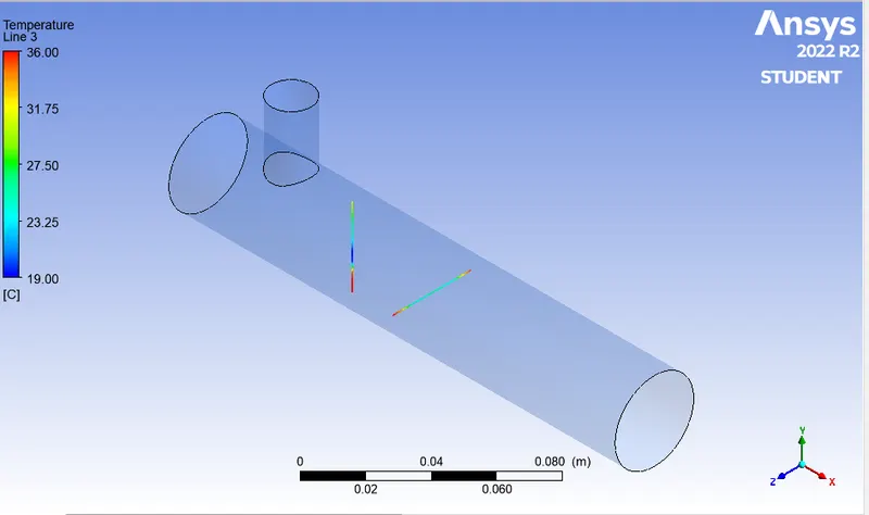
vi) Temperature line plot across the length of the pipe
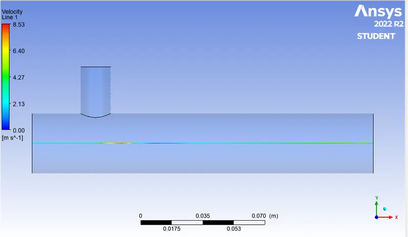
vii)Velocity line plot along the length of the pipe
viii) Velocity line plot across the length of the pipe
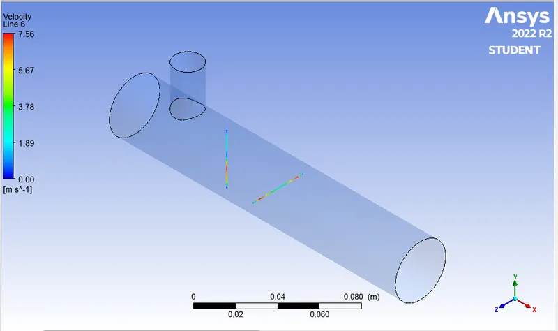
Which model to be perform k-ℇ realizable and k-Ω SST model?
K- epsilon realizable model:
It provides the improved predictions for the spreading rate of both planer and round jets.
It is ideal for the prediction flow behavior in the regions away from the wall.
K- omega SST model:
It’s a hybrid model combining the Wilcox K-omega and K-Epsilon model
The K- omega SST turbulence model is a two equation eddy viscosity model that is used for many aerodynamics applications
It provides the more accurate prediction of flow separation than other RNS model.
The shear stress limiter helps the K- omega model to avoid the build-up of excessive turbulent kinetic energy near the stagnation points.
The SST model exhibit the less sensitivity to free stream conditions than many other turbulence model.
K- omega SST should be robust enough to model most of the engineering applications.
Thus as per my consern is to go with K- omega SST model.
Case study 3:
Parameters for the case study 3 is in the below table.
| Type of Tee | Short Tee |
| Moment ratio | 4 |
| Hot air velocity and Temperature | 3 m/s, 360C |
| Cold air velocity and Temperature | 12 m/s, 190C |
| Total elements or cell count | 510147 |
| Turbulance model | k-Ω SST |
| Theoritical temperature mixture as per calculated |
280C |
For the above boundry condition following results are obtained.
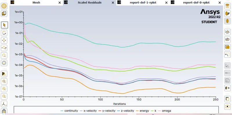
i) Residuals plot
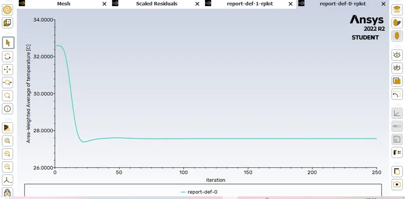
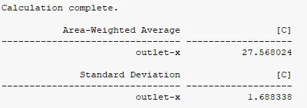
ii) Area-weighted-Average of temperature
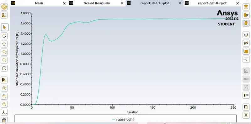
iii) Standard deviation
iv) Result
Post processor results
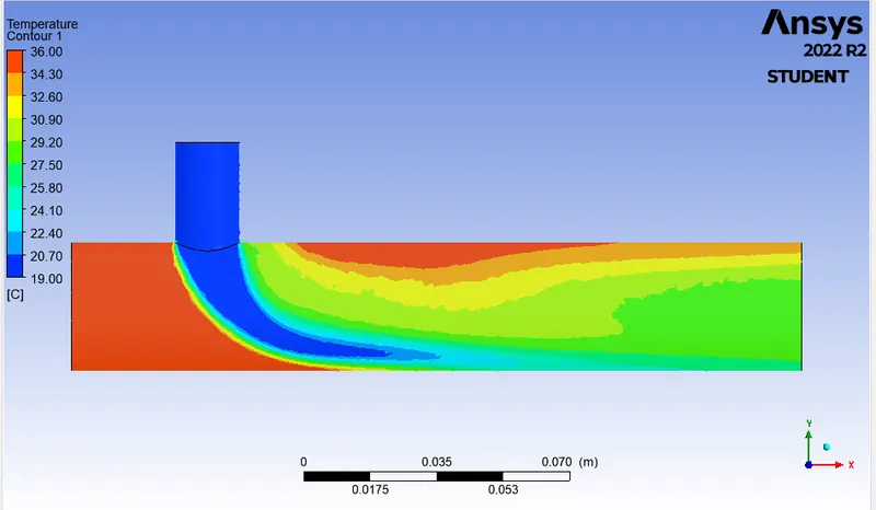
i) Temperature contours plot along the length of the pipe
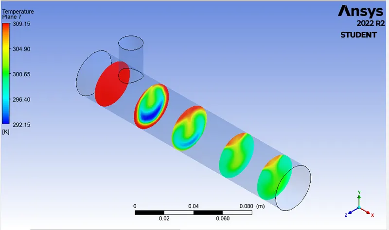
ii) Temperature contours plot across the length of the pipe
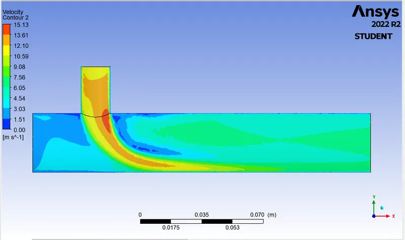
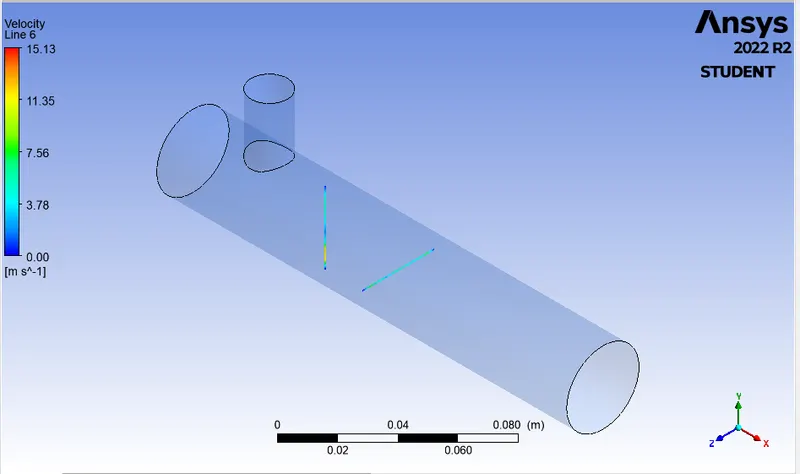
iii) Velocity contours plot along the length of the pipe
iv) Velocity contours plot across the length of the pipe
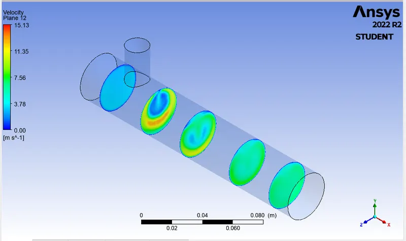
v) Temperature contours plot along the length of the pipe
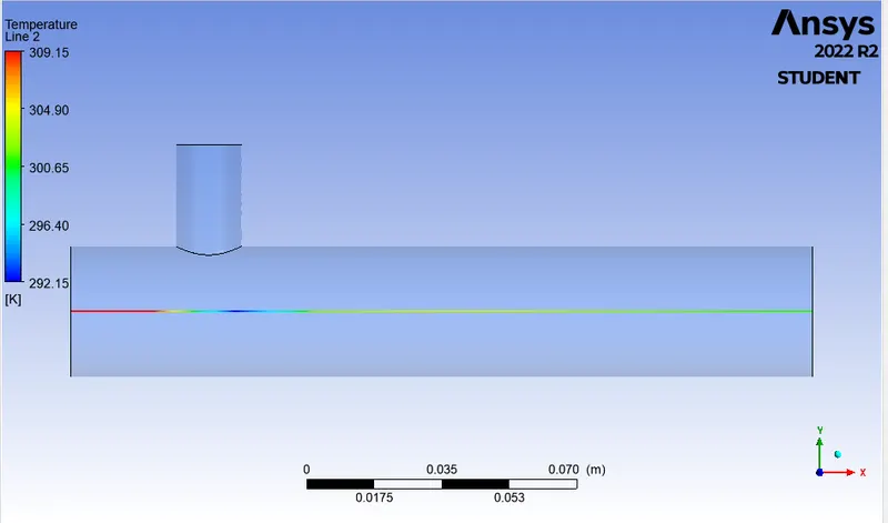
vi) Temperature contours plot across the length of the pipe
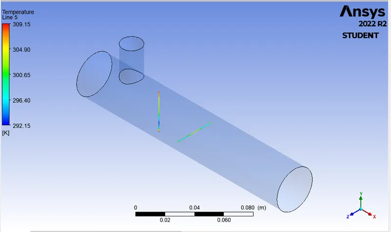
vii)Velocity contours plot along the length of the pipe
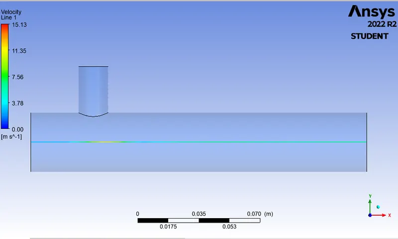
viii) Velocity contours plot across the length of the pipe
Case study 4:
Parameters for the case study 4 is in the below table.
| Type of Tee | Long Tee |
| Moment ratio | 2 |
| Hot air velocity and Temperature | 3 m/s, 360C |
| Cold air velocity and Temperature | 6 m/s, 190C |
| Total elements or cell count | 504561 |
| Turbulance model | k-Ω SST |
| Theoritical temperature mixture as per calculated |
30.7690C |
For the above boundry condition following results are obtained.
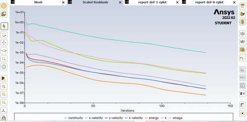
i) Residuals plot
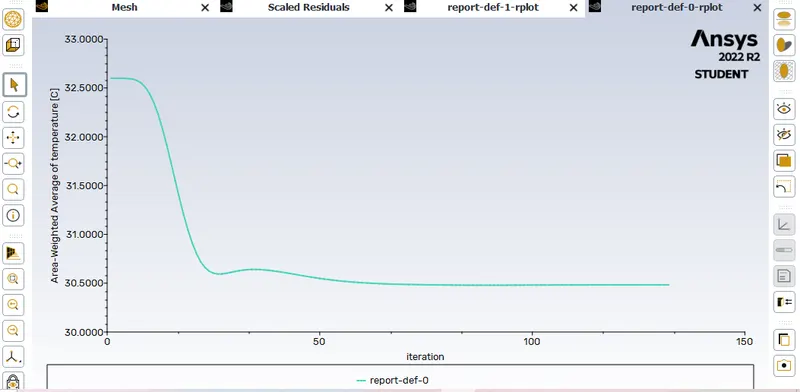
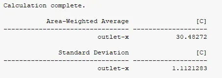
ii) Area-weighted-Average of temperature
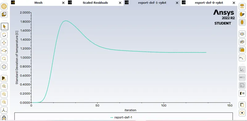
iii) Standard deviation
iv) Result
Post processor results
i) Temperature contours plot along the length of the pipe
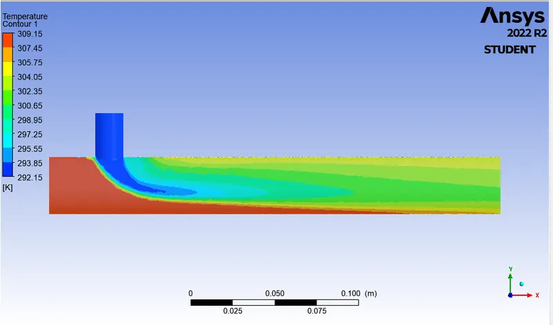
ii) Temperature contours plot across the length of the pipe
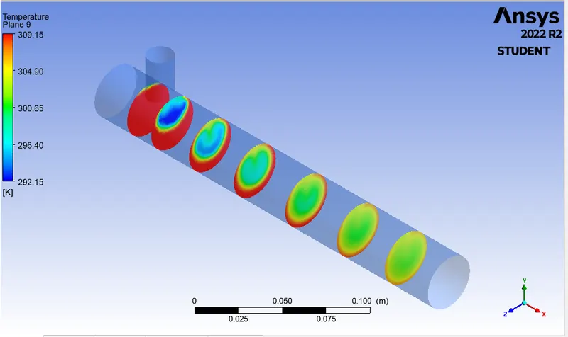
iii) Velocity contours plot along the length of the pipe
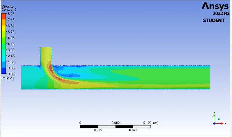
iv) Velocity contours plot across the length of the pipe
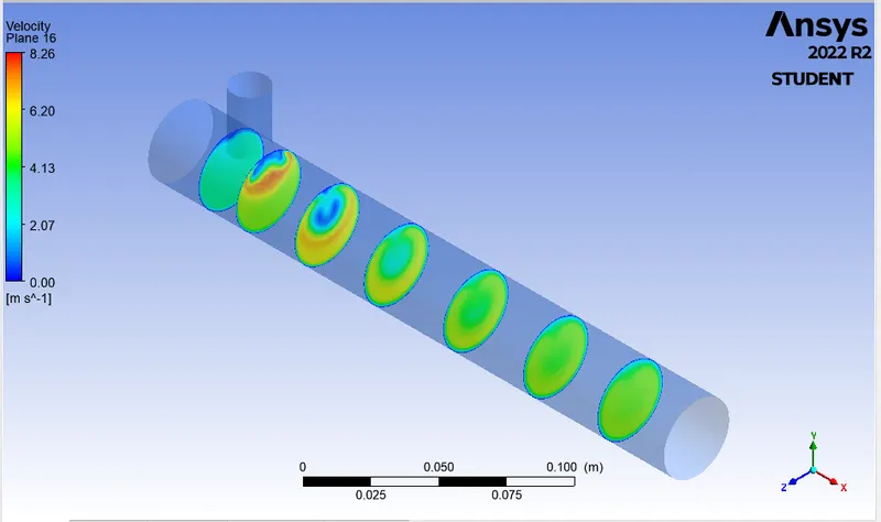
v) Temperature contours plot along the length of the pipe
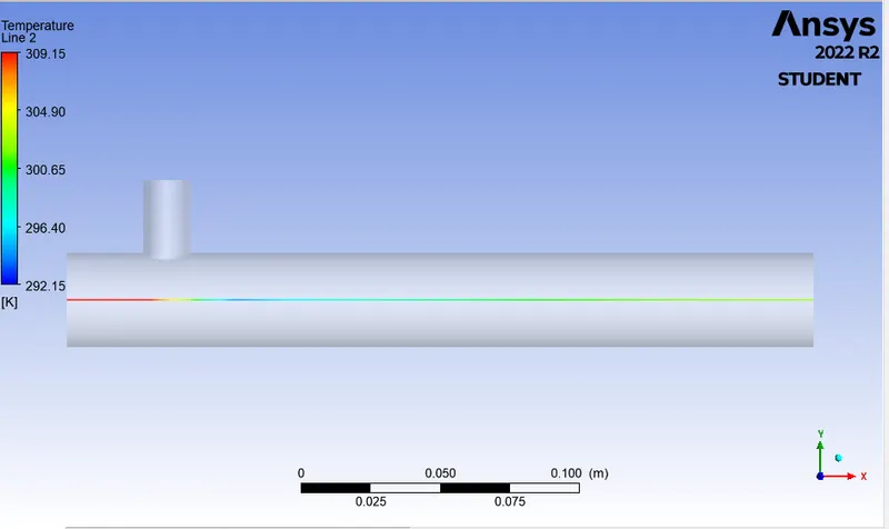
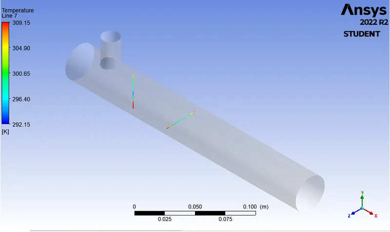
vi) Temperature contours plot across the length of the pipe
vii)Velocity contours plot along the length of the pipe
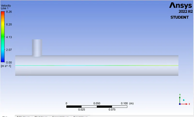
viii) Velocity contours plot across the length of the pipe
Case study 5:
Parameters for the case study 5 is in the below table.
| Type of Tee | Long Tee |
| Moment ratio | 4 |
| Hot air velocity and Temperature | 3 m/s, 360C |
| Cold air velocity and Temperature | 12 m/s, 190C |
| Total elements or cell count | 504561 |
| Turbulance model | k-Ω SST |
| Theoritical temperature mixture as per calculated |
280C |
For the above boundry condition following results are obtained.
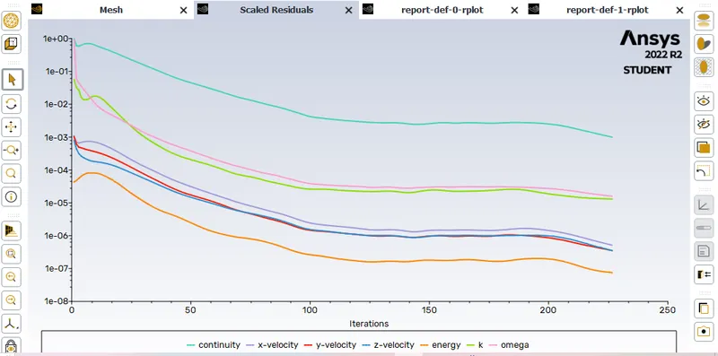
i) Residuals plot
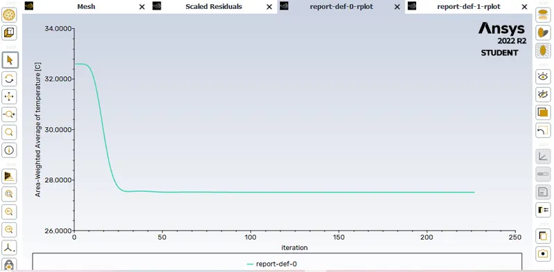
ii) Area-weighted-Average of temperature
iii) Standard deviation
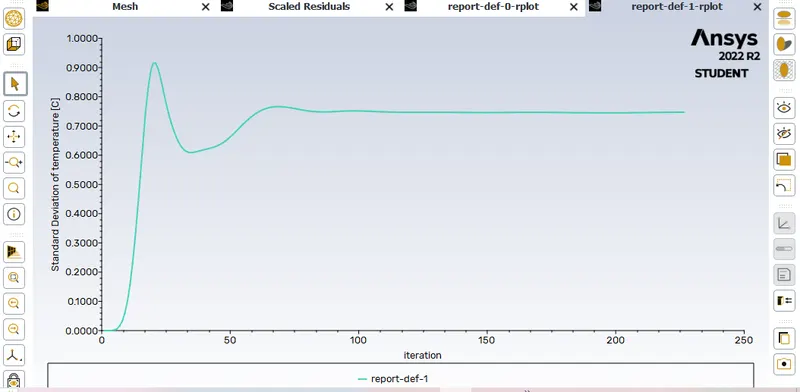
From the above graph it is understod that as the itiration increases the we are getting towards accurate results and after the itirations of 100 the convergence takes place.
iv) Result
Post processor results
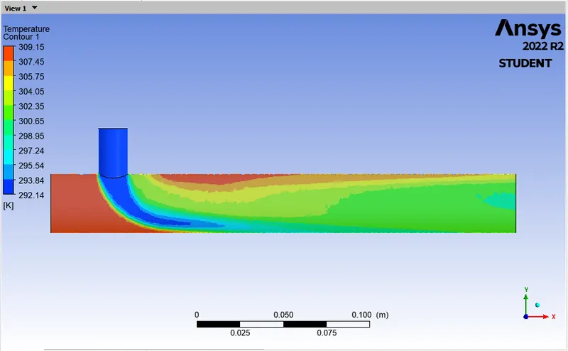
i) Temperature contours plot along the length of the pipe
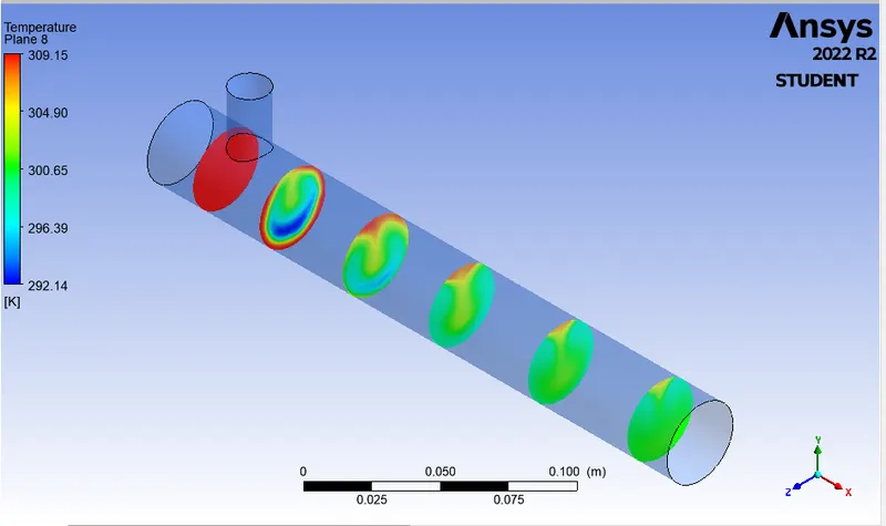
ii) Temperature contours plot across the length of the pipe
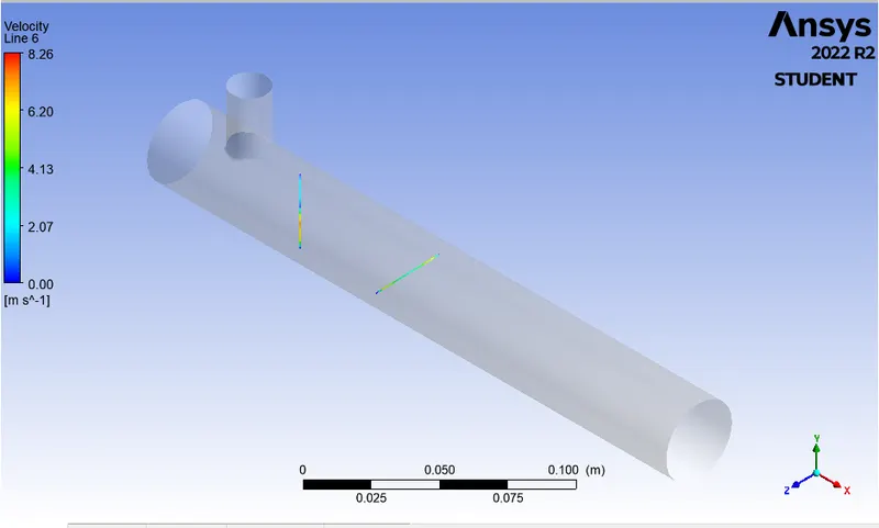
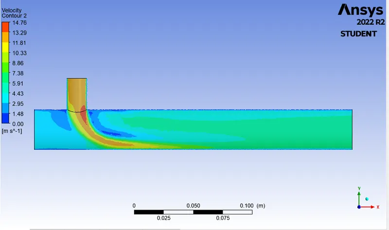
iii) Velocity contours plot along the length of the pipe
iv) Velocity contours plot across the length of the pipe
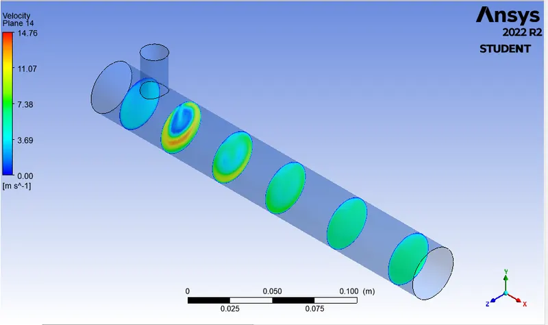
v) Temperature contours plot along the length of the pipe
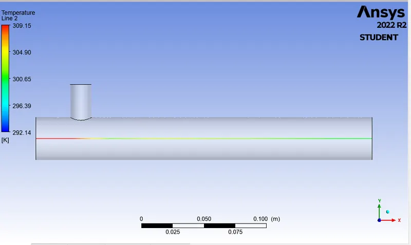
vi) Temperature contours plot across the length of the pipe
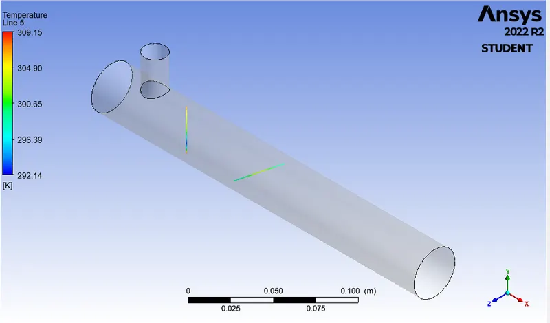
vii)Velocity contours plot along the length of the pipe
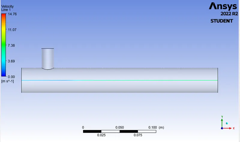
viii) Velocity contours plot across the length of the pipe
Convergency study:
For each case of simulation 250 iterations were performed as it proved sufficient to satisfy the convergence criteria. There are no universal metrics for judging convergence. Residual definitions that are useful for one class of problem are sometimes misleading for other classes of problems. Therefore, area weighted average of temperature and standard deviation of temperature is also monitored at outlet. For most problems, the default criterion in ANSYS Fluent is sufficient. This criterion requires scaled residuals decrease to 10e- 3 or less for all equations except energy equation, for which the criterion is 10e-6 . But it can be observed from the following graphs of residuals that the energy equation has not reached the convergence criterion, this is because the temperature difference between input values and output is very less. It is observed that the residuals haven’t reached the convergence criterion but still the solution is converged as for more than 50 iterations the graph shows same behaviour at the end of graph. Also, the graph of area-weighted average of temperature and standard deviation of temperature at outlet show same behaviour for more than 50 iterations. Hence, we can confirm the convergence of solution by observation.
Post processor description:
Post processing is necessary for creating and investigating the behaviour of output results throughout the body. After the simulation, the results are examined and analysed through CFD-Post to verify the results and conclusions drawn on the obtained results. Contour plots for temperature and velocity are observed for all the cases which provide a visual of actual process. It can be observed in the temperature plot the contours of high temperature represented by colour red are present in case study 1 case study 2 and case study 4 represented. This indicates that there is high temperature at outlet, but it is not for case study 3 and case study 5. It can be observed from the contour plot of velocity that velocity at outlet in Case study 3 and Case study 5 is relatively greater than that of other case. Hence, the simulation results can be confirmed based on visuals obtained by post processing.
Results and discussion:
| Case study | Type of Tee | Turbulance model | Total cell count/Elements | Inlet-Y Temperature | Inlet-Y Velocity | Inlet-X Temperature | Inlet-X Velocity | Momentum Ratio | Analytical Temperature value from i and ii calculated above | Area-weighted-Average of temperature as per CFD results | Standard deviation of temperature as per CFD results | Number of Iterations |
|
1 |
Short-Tee | k-ℇ realizable | 510147 |
190C |
3 m/s | 360C | 6 m/s | 2 | 32.3430C | 30.40890C | 1.814190C | 250 |
| 2 | Short-Tee | k-Ω SST | 510147 | 190C | 3 m/s | 360C | 6 m/s | 2 | 32.3430C | 30.51190C | 1.835360C | 250 |
| 3 | Short-Tee | k-Ω SST | 510147 | 190C | 3 m/s | 360C | 12 m/s | 4 | 280C | 27.56800C | 1.688330C | 250 |
| 4 | Long-Tee | k-Ω SST | 504561 | 190C | 3 m/s | 360C | 6 m/s | 2 | 32.3430C | 30.48270C | 1.11210C | 250 |
| 5 | Long-Tee | k-Ω SST | 504561 | 190C | 3 m/s | 360C | 12 m/s | 4 | 280C | 27.51790C | 0.747040C | 250 |
From the above table it is clearly says that Case study 3 and Case study 5 both ( for momentum ratio 4 ) are more mixing efficiency than any other case study which is highlighed by green colour in the above result table.
Conclusion:
From the result of area weighted-average of temperature at outlet it can observed that the temperature at outlet shows no significant change when the velocity is same even though the length of outlet is increase from the junction. But it has been observed that the outlet temperature shows significant decrease when momentum ratio is increased resulting in increased mixing efficiency. The above-mentioned behaviour is also same for the results of standard deviation of temperature at outlet. Hence, based on obtained results and observations made, Case study 3 and Case study 5 yields more mixing efficiency relative to other cases. Also, the increase in length of tee does not play any significant role as compared to increase in momentum ratio on the efficiency of Mixing tee.