Week 3 - External flow simulation over an Ahmed body.
AIM: External flow simulation over an Ahmed body by using Air as working fluid with the velocity of 25 m/s
OBJECTIVE:
Following are the expected Results after sovling and obtain the results of simulation.
1. Velocity and pressure contours.
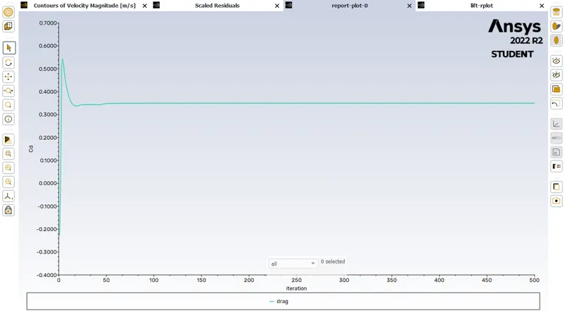
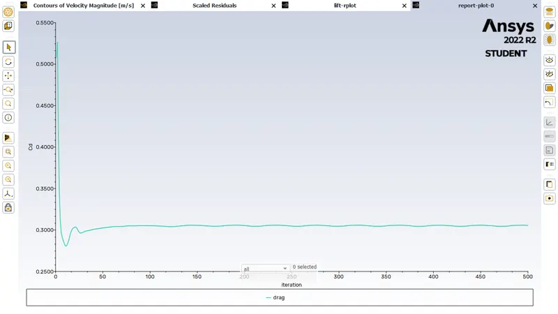
2. The drag coefficient plot for a refined case. ( For velocity of 25m/sec, the drag coefficient should be around 0.33).
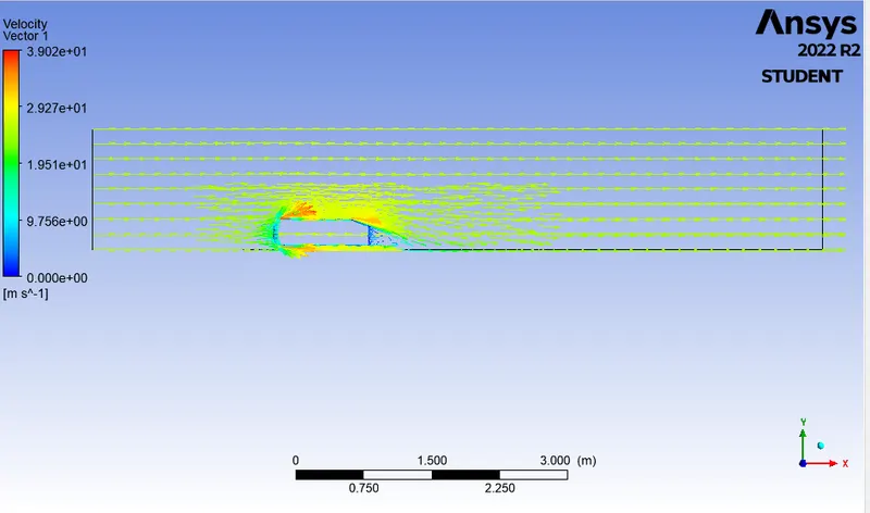
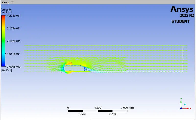
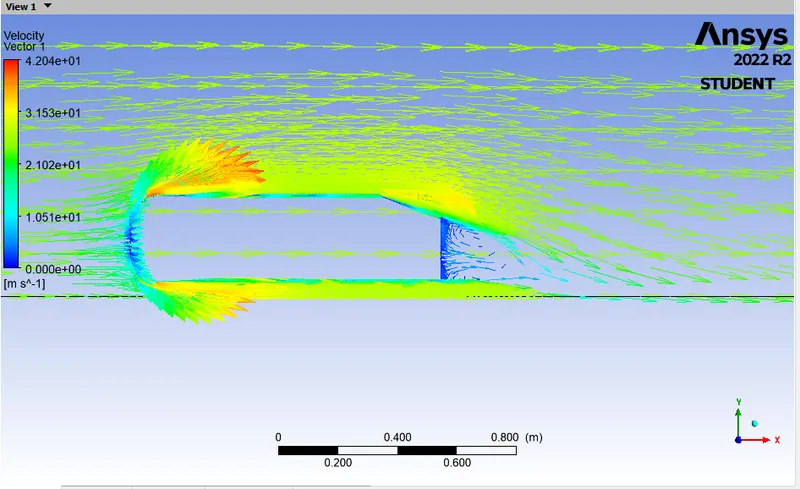
3. The vector plot clearly showing the wake region.
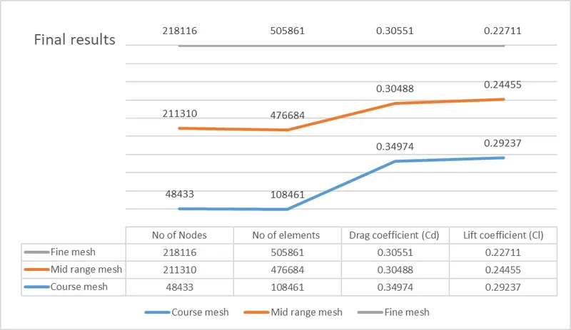
4. Perform the grid independency test and provide the values of drag and lift with each case.
THEORY:
What is Ahmed's body and its importance?
Before going to Ahmed's body stright away let us know about road vehicle models. The road vehicle models most commonly used are Ahmed body (Ahmed et al., 1984), Windsor body (Pavia et al., 2018), and Lorry model (Dalla Longa et al., 2019). These models oftentimes lack details such as side mirror and wheels, but they adequately capture the essential flow characteristics of a real vehicle. Most importantly, the wake behind these models is comparable to the wake that would have been generated behind a real road vehicle. This allows researchers to conduct fundamental studies regarding the wake of a road vehicle which in turn provide valuable information for engineers to design an aerodynamically efficient vehicle.
Please refer the below photo for the different road vehicle models

(a)Ahmed body, (b) Lorry model, (c) Windsor model
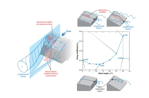
The Ahmed body model is utilized in this study. The Ahmed body was introduced in 1984 by Ahmed, Fantin and Ram (Ahmed et al., 1984). They introduced the model to study the wake topology of a ground vehicle with varying afterbody configuration. The drag coefficient as well as the wake topology varied significantly with rear slant angle alpha as shown in road vehicle models figures (a) . The minimum and maximum drag occurred when alpha ≈ 12.5 ºand alpha ≈ 30.0º, respectively. The increase in drag is attributed with the emergence of the counter rotating longitudinal vortices called the C-pillar vortices. These vortices increase the three dimensionality of the wake which in turn increases the drag. The separation point of the flow greatly influences the wake topology as well as drag experienced by the body. There is two possible separation points since the fluid can either separate at the top slant edge or bottom slant edge. The lower drag coefficient is associated with separation at the top slant edge since it prevents the C-pillar vortices from developing.
Please refer the below diagram for the Wake topology of an Ahmed body
Why negative pressure at the wake region?
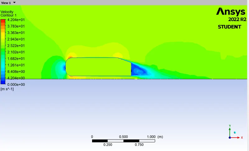
The velocity contours extending behind the body indicate the low velocity wake region, which causes the form drag. As the wake area is reduced, the drag-causing eddies (vortices), generated due to the pressure difference between the top and bottom of the Ahmed body at the rear trailing end, come closer together. This result in less kinetic energy being dissipated due to these smaller eddies and consequently less compensation power required by the engine to propel the vehicle forward. It additionally results in higher pressure being applied at the rear surface of the body and consequently less form drag.
What is the significance of the point of separation?
The point of separation defined by the Ahmed body and the flow, the alpha angle depending on which value is at it causes change in flow direction, forces required, lift on the body, induced drag due to “tip vortex”, at a critical value flow in slant stalls and reduced lift-reducing as well drag, all depending on the value of alpha and the Reynolds number.
What is y+ and its significance?
Near the wall modelling it is well-known that the mesh size should be small enough, however then the question follows is how small ? Thus, here comes the concept of y+, and based on the y+ value the first cell height can be calculated. We have to under stand the concept of boundary layer especially turbulent boundary layer. In a flow bounded by a wall, different scales and physical processes are dominant in the inner portion near the wall, and the outer portion approaching the free stream. These layers are typically known as the inner and outer layers. Considering the flow over a smooth flat plate the boundary layer can be distinguished into two types namely laminar boundary layer and turbulent boundary layer. Since we are dealing with the turbulent boundary layer let us not get into the laminar boundary layer. Typical boundary layer structure over a flat plate is shown below. In between the laminar and turbulent boundary layer there lies a transition region. Typically for flow over a flat plate the transition usually occurs around Reynolds number(Re~5X10^5).
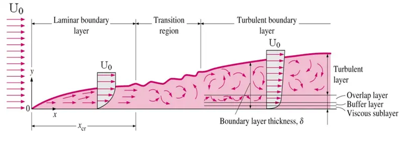
From the above figure it can be seen that in turbulent boundary layer region flow near the wall has been analysed in terms of three layers:
- The inner layer, or sublayer, where viscous shear dominates
- The outer layer, or defect layer, where large scale turbulent eddy shear dominates
- The overlap layer, or log layer, where velocity profiles exhibit a logarithmic variation
A still clear image of the above is shown below
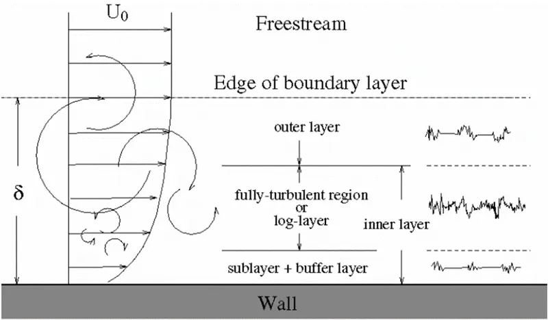
where U0 is the free stream velocity and delta is the boundary layer thickness, y is the vertical distance measured from the wall.
Turbulent boundary layers are usually described in terms of several non-dimensional parameters. The boundary layer thickness, is the distance from the wall at which viscous effects become negligible and represents the edge of the boundary layer.
Turbulent boundary layers are usually described in terms of several non-dimensional parameters. The boundary layer thickness, delta is the distance from the wall at which viscous effects become negligible and represents the edge of the boundary layer.
Schematic diagram of general law of wall is shown below:
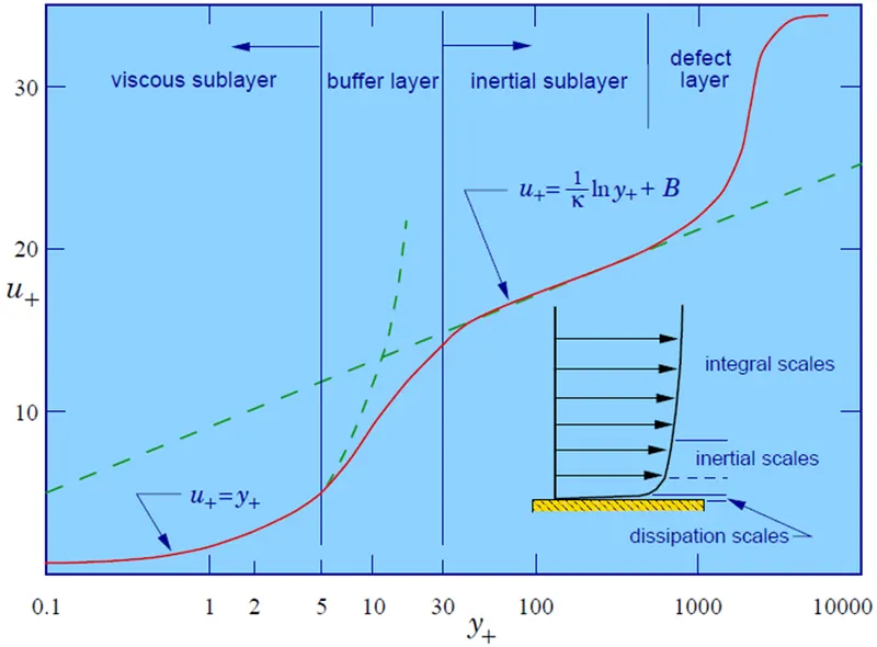
The near-wall modelling significantly impacts the fidelity of numerical solutions, inasmuch as walls are the main source of mean vorticity and turbulence. After all, it is in the near-wall region that the solution variables have large gradients, and the momentum and other scalar transports occur most vigorously. Therefore, accurate representation of the flow in the near-wall region determines successful predictions of wall-bounded turbulent flows.
Theoritical y+ calculation:
i) Reynolds number:
Reynolds number is a dimensionless quantity that is used to determine the type of flow pattern as laminar or turbulent while flowing through a pipe. Reynolds number is defined by the ratio of inertial forces to that of viscous forces. It is givan by the below equation.
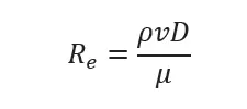
Where Re is the Reynolds number, ρ is the density of the fluid (kg/m³), V is the velocity of flow (m/s), D is the pipe diameter or length of the ahemed body here (m), μ is the viscosity of the fluid (kg/m-s).
Please refer the below table for the input parameters
| ρ is the density of the fluid (kg/m³) | 1.225 |
| V is the velocity of flow (m/s) | 25 |
| D is the pipe diameter or length of the ahemed body here (m) | 1.044 |
| μ is the viscosity of the fluid (kg/m-s) | 1.789X10^-5 |
Applying these values in the Re equation
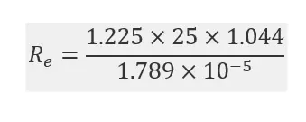
Therefore we obtain the Reynolds number as 1787171.60424
Skin-Friction Drag and Skin-Friction Coefficient (Cf):
Skin friction drag is a type of aerodynamic or hydro dynamic, which is resistant force exerted on an object moving in a fluid. Skin friction drag is caused by the viscosity of fluids and is developed from laminar drag to turbulent drag as a fluid moves on the surface of an object. Skin friction drag is generally expressed in terms of the Reynolds number. The skin friction coefficient is a dimensionless skin shear stress which is nondimensionalized by the dynamic pressure of the free stream. The skin friction coefficient is defined at any point of a surface that is subjected to the free stream.The skin friction coefficient is a strong function of the Reynolds number  , as increases
  decreases.
Theoritically it is given by
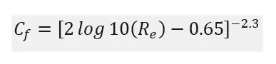
By taking the above Re value calculated and find the Cf value
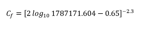
we obtain the Skin-Friction Coefficient (Cf) value as 3.389X10^-3
Wall Shear Stress (τw):
Wall shear stress expresses the retarding force (per unit area) from a wall in the layers of a fluid flowing next to the wall. It is given by the below equation
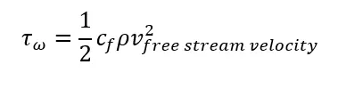
By taking the above Cf value and others paramerer valuesfrom the table calculated and find the value of Wall Shear Stress
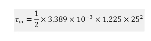
we obtain the Wall Shear Stress (τw) value as 1.2973 pascal (Pa)
Friction Velocity (U*):
Shear velocity, also called friction velocity, is a form by which a shear stress may be re-written in units of velocity. It is useful as a method in fluid mechanics to compare true velocities, such as the velocity of a flow in a stream, to a velocity that relates shear between layers of flow. It is given the the equation
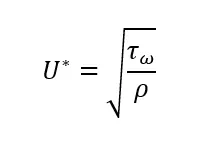
By solving the equation by putting the above calculated values.
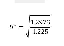
we obtain the Friction Velocity (U*) value as 1.02908 m/s
Wall Distance (y):
Wall distance (y) is the vertical distance measured from the wall as previously discussed in the y+ and its significance. It is given by the equation
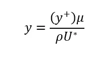
Here we have to maintain the Y+ value wit respect to the turbulance model
For RNS model of K- epsalon, the range of y+ with is 30-300
For K-omega-SST model the range of y+ is 0-5.
In this case we are using K-omega-SST so taken y+ as 5
By putting the respective values in the above equation
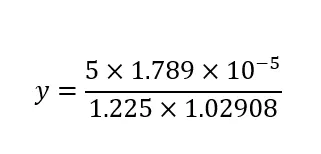
we obtain the Wall Distance (y) value as 7.0956X10^-5 m
SST model is known as one of the more accurate turbulence model for separation prediction compared to k−ε and k −ω formulations. SST model combines the strengths of k −ω in the boundary layer and gradually switches to a k −ε formulation in the outer part of the boundary layer to liberate from freestream dependency of the k −ω model. The blending between k − ε and k − ω formulations is ensured with the F1 blending function. This model is sensitized to adverse pressure gradient by taking into account the shear stress transport, modifying the eddy viscosity formulation in the boundary layer of the model, with the blending function F2.
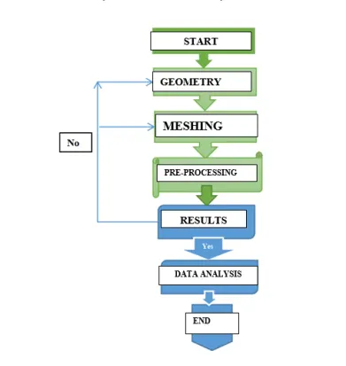
Please refer the below chrt for the CFD work flow analysis of the Ahmed body
Geometry setup of Ahmed body:
The Ahmed’s body reference geometry is composed by three parts: the front section, which is rounded to keep the flow attached to the surface; the central section, represented by a rectangular box with sharp edges; and the back inclined surface, where the flow shows different behaviors, according to the angle of inclination.
Please refer the below photo for the Ahmed body model and geometry.
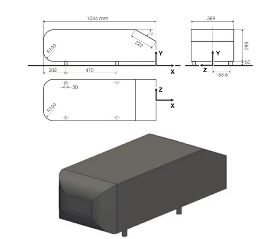
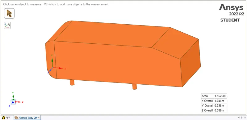
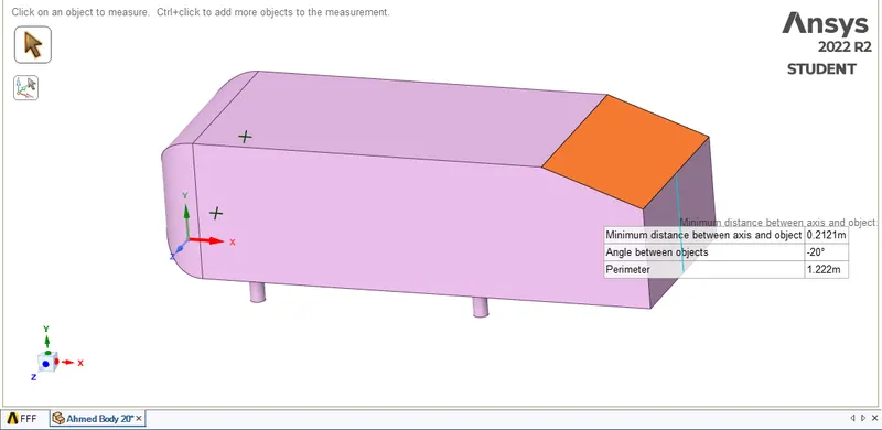
The overall length, width and height of the Ahmed body model is 1.044 m, 0.389 m and 0.338 m respectively as shown in the above. Ahmed body with the 20 degree slant angle.
In the geometry setup we have the following steps.
Step 1: Splitting the geometry by using split comand
Before the spliting we have to insert a plane at the center of the body at XY plane as shown in the below
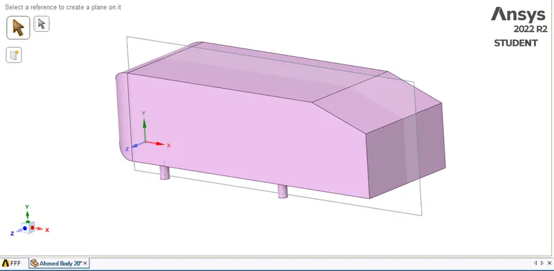
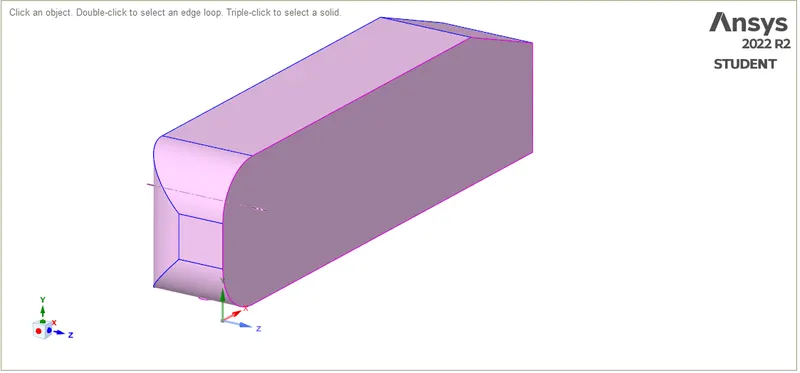
Splitted body is as shown in the below, to save the simulation time we are splitting the body and simulating it.
Step 2: Creating an enclosure two enclosures to the Ahmed body
The computational domain larger enclosure starts 2m in front of the model and extends to 5m behind the model. The width of the domain is 0.5 m and its height is 1 m
The computational domain smaller enclosure starts 1m in front of the model and extends to 2m behind the model. The width of the domain is 0.25 m and its height is 0.5 m
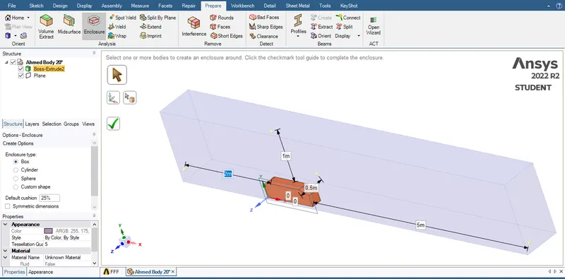
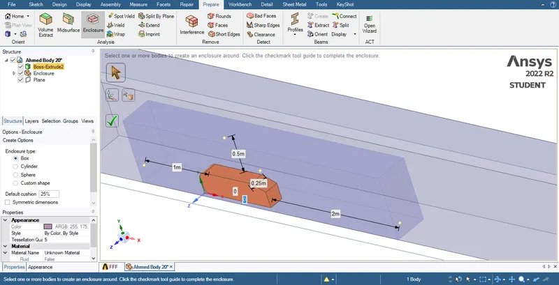
Step 3: Checking for the interference
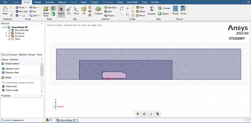
There is a overlap in the enclosure 2 as shown in the below, Go to prepare and interference the surface and click ok
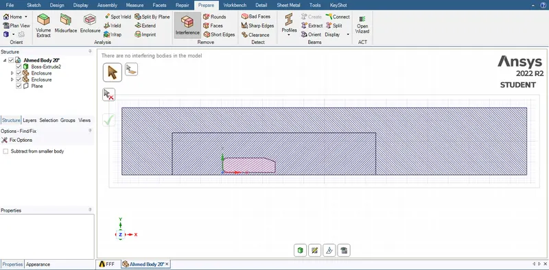
Please refer the below photo for after interference done.
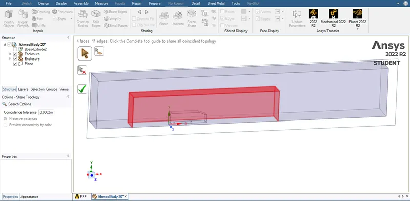
Step 4:Shearing the topology
Go to workbench and shear the topology as shown belw and click green colour tick mark.
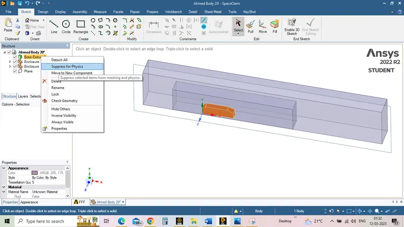
At last supress the Boss-Extrude2 for physics as shown in the below.
Meshing:
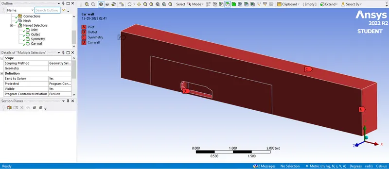
Before going for meshing we have to nomenclature the geometry setuped model as inlet, outlet, symmetry and car wall as shown in the below
We are studying the 3 types of meshes mainly course mesh, mid-range mesh and fine mesh.
Following are the inputs to all the 3 types of meshs

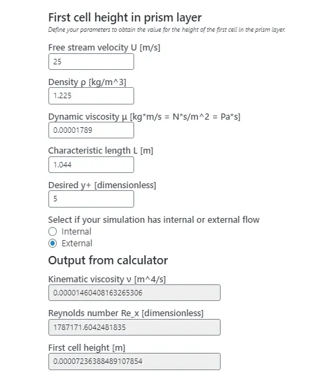
Calculation of first cell heigt in prism layer online by y+ calculator as shown below the first cell height is 0.00007236 m, prisem layer stretching is 1.2 and by maintaining the prism layer total thickness grater then or equal to the boundary layer thickness number of prisem layers obtained is 23.
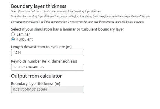
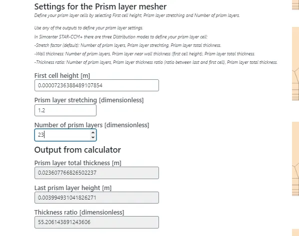
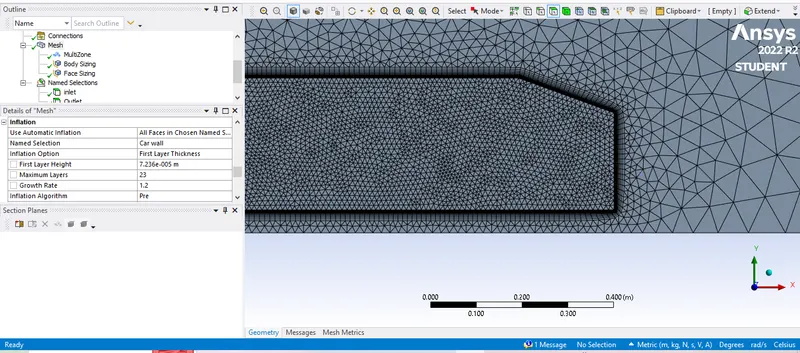
By applying these values in the inflation we obtain as below.
1) Course mesh:
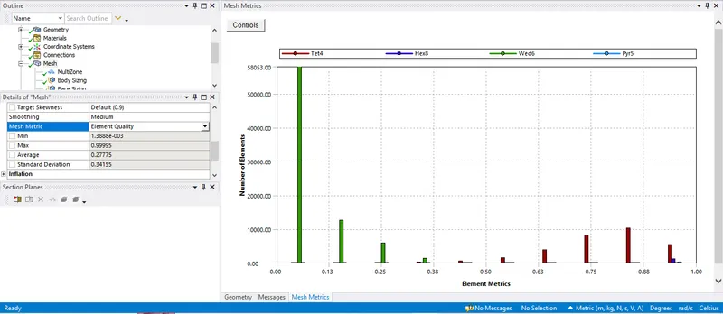
Please refer the below for the course mesh obtained and number of nodes and elements obtained are 48433 and 108461 respectively.
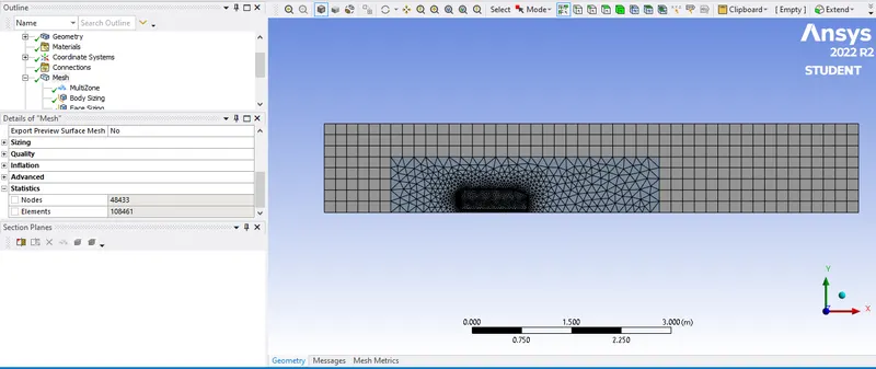
Please refer the below for the mesh elemental quality obtained and average value is 0.27775
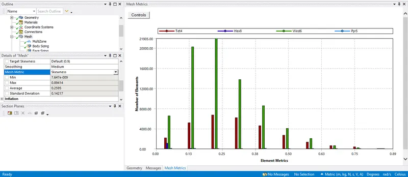
Please refer the below for the Skewness obtained and average value is 0.2595
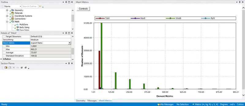
Please refer the below for the Aspect ratio obtained and average value is 73.037
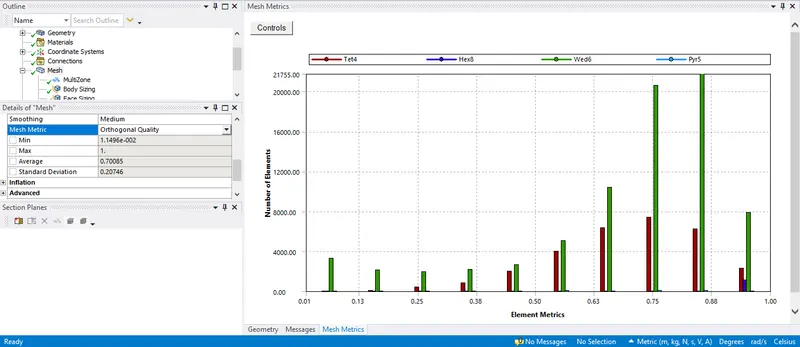
Please refer the below for the Ortogonality obtained and average value is 0.70085
2) Mid range mesh:
Please refer the below for the course mesh obtained and number of nodes and elements obtained are 211310 and 476684 respectively.
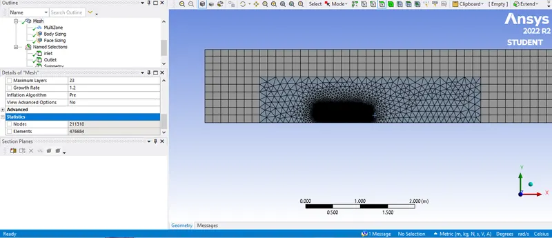
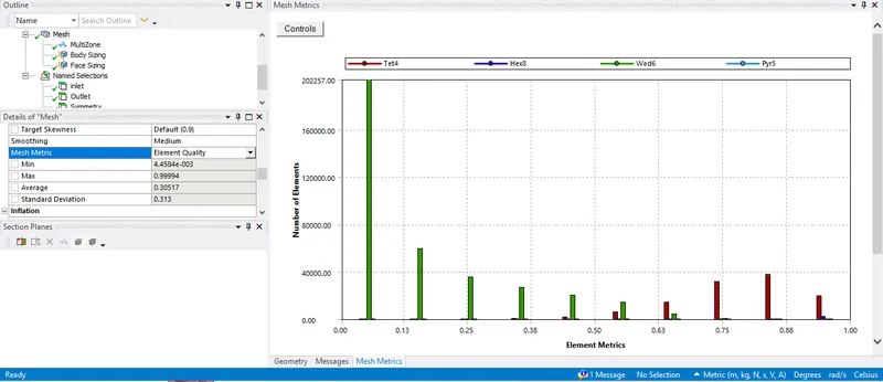
Please refer the below for the mesh elemental quality obtained and average value is 0.30517
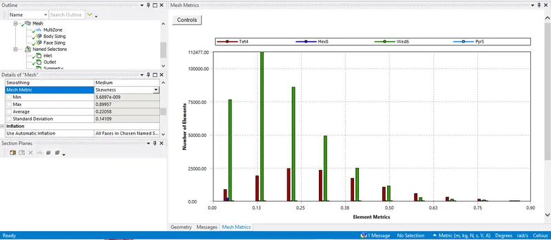
Please refer the below for the Skewness obtained and average value is 0.22058
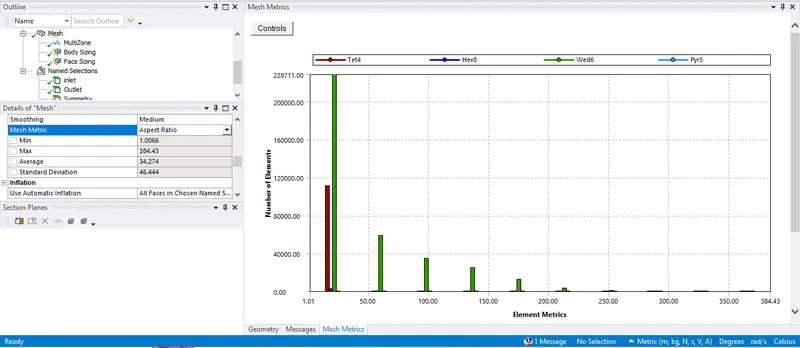
Please refer the below for the Aspect ratio obtained and average value is 34.274
Please refer the below for the Ortogonality obtained and average value is 0.76716
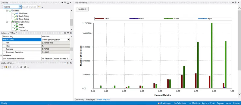
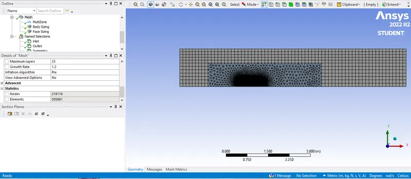
3) Fine mesh:
Please refer the below for the course mesh obtained and number of nodes and elements obtained are 218116 and 505861 respectively.
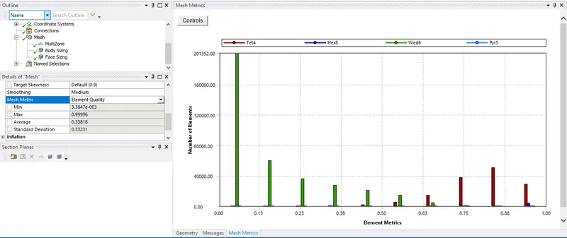
Please refer the below for the mesh elemental quality obtained and average value is 0.33818
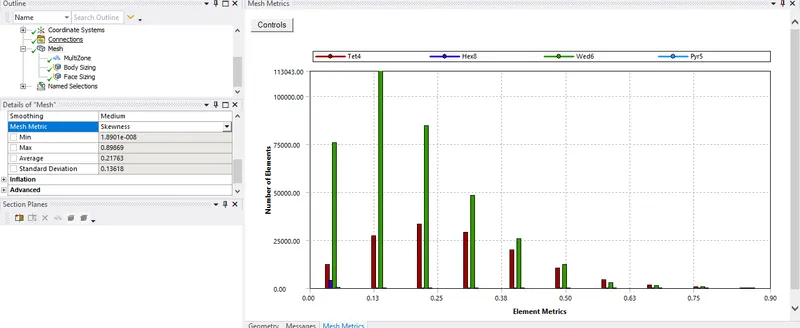
Please refer the below for the Skewness obtained and average value is 0.21763
Please refer the below for the Aspect ratio obtained and average value is 32.505
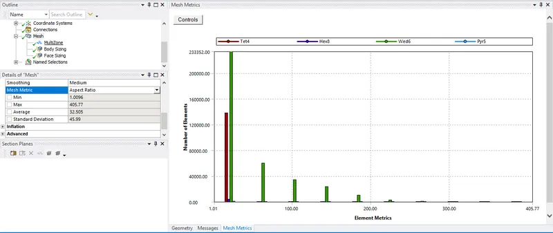
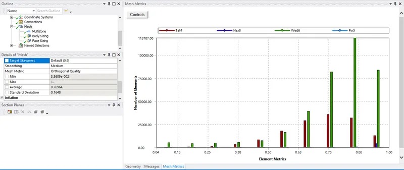
Please refer the below for the Ortogonality obtained average value is 0.76964
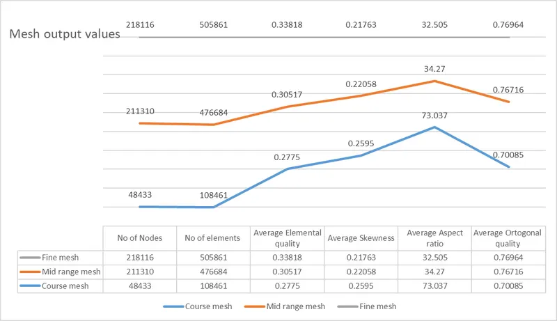
From the above graph we can conclude that as the mesh element size decreases the increase in the no of nodes and elements, elemntal quality and ortogonal quality but decrease in the Skewness and aspect ratio.
Pre processer solver setup or Fluent setup:
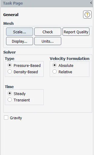
Please refer the below table for the fluent setup applied to solve the problem.
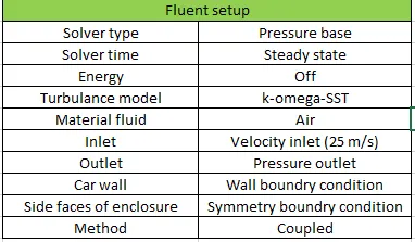
Please refer the below photo for solver applied.
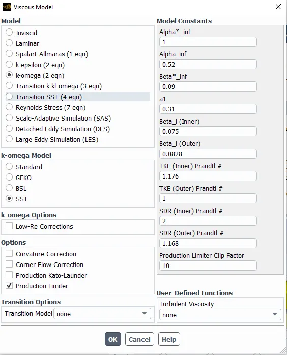
Please refer the below photo for the Turbulance model applied
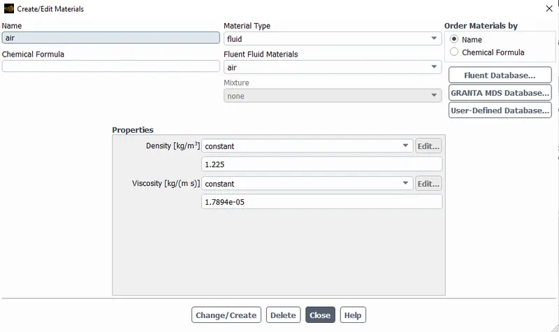
Please refer the below photo for the Material used.
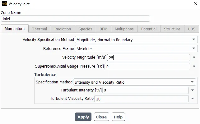
Please refer the below photo for the Velocity inlet applied.
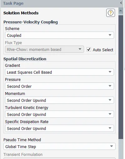
Please refer the below photo for the Coupled method applied.
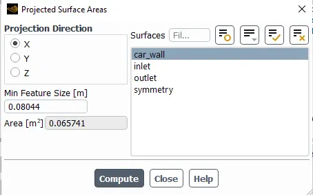
Please refer the below photo for the Car wall area obtained.
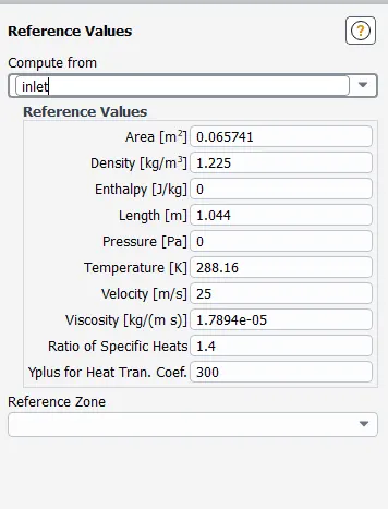
Please refer the below photo for the Reference value applied.
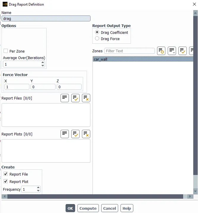
Drag and lift report defination will be done as shown below
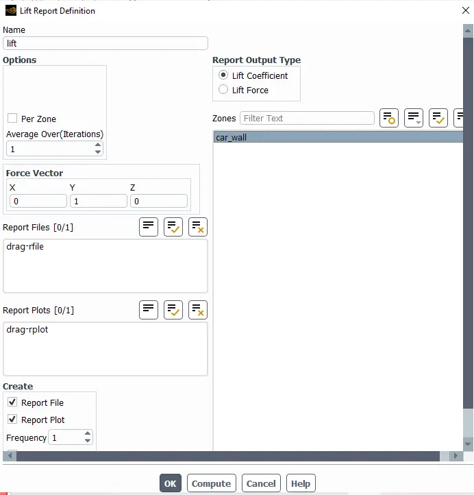
After given these inputs hybrid initialization will be done followed by calculation by giveing 500 itirations.
Post processer or Results :
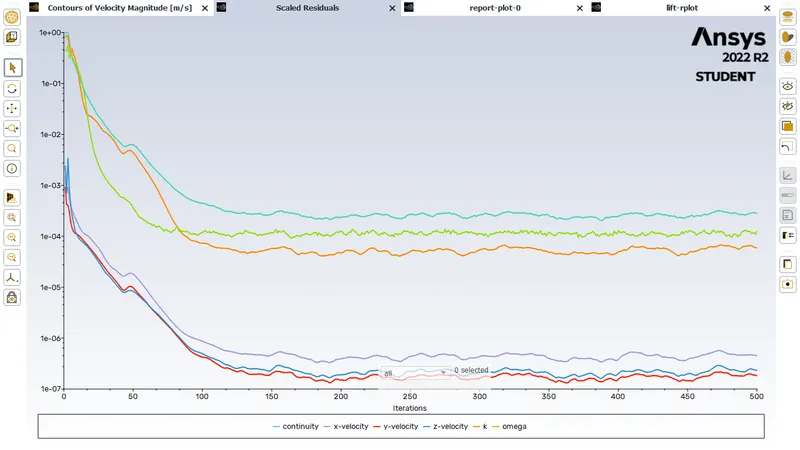
1) Following results are obtained for the course mesh
Please refer the below photo for the Residuals plot
Please refer the below photo for the drag plot
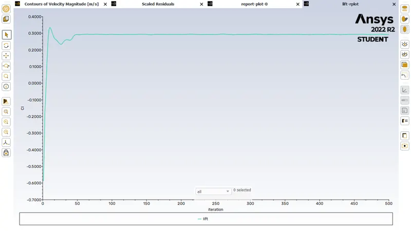
Please refer the below photo for the lift plot
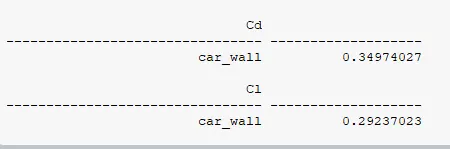
Please refer the below photo for the drag and lift coefficent value obtained
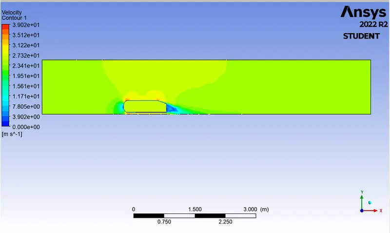
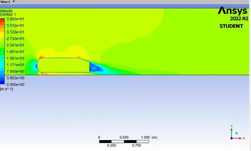
Please refer the below photo for the Velocity countor
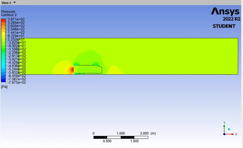
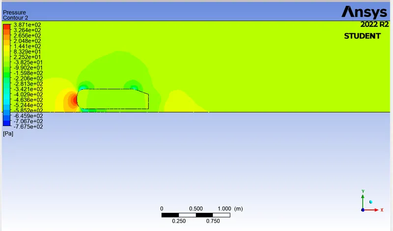
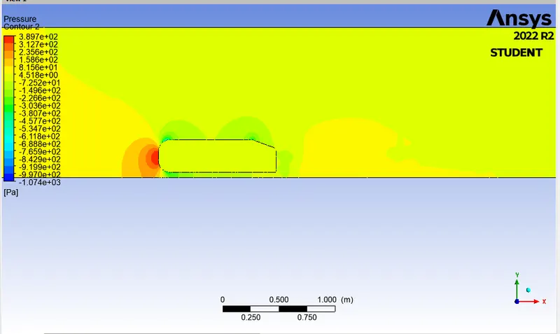
Please refer the below photo for the Pressure countor
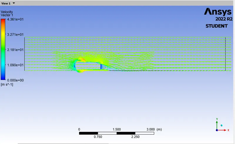
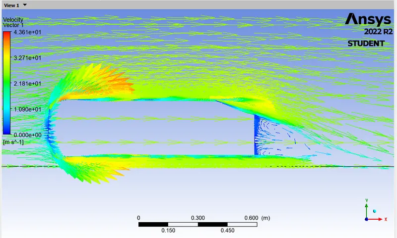
Please refer the below photo for the Velocity vector
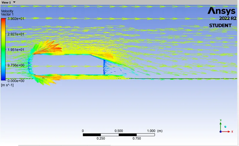
2) Following results are obtained for the mid-range mesh
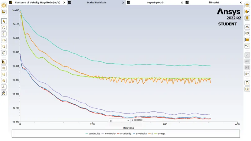
Please refer the below photo for the Residuals plot
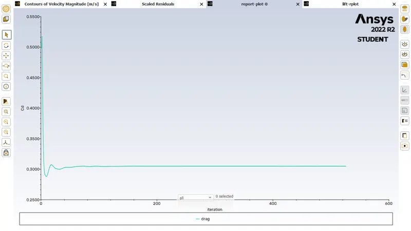
Please refer the below photo for the drag plot
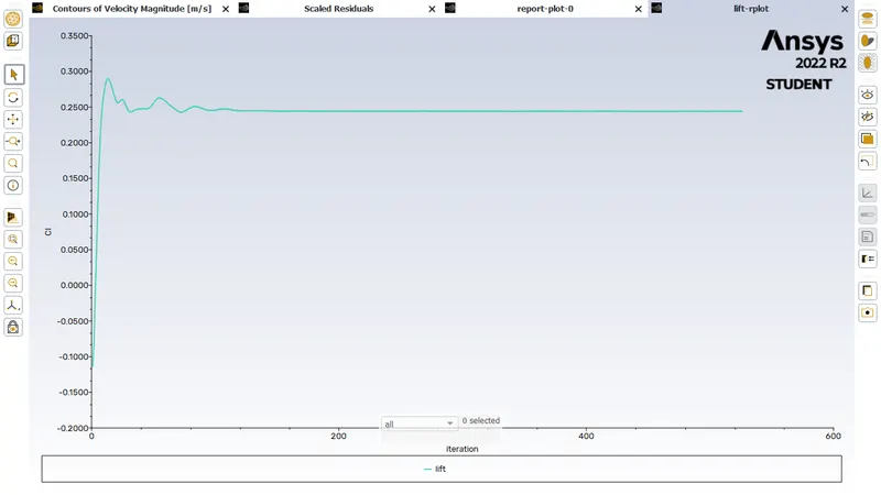
Please refer the below photo for the lift plot
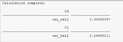
Please refer the below photo for the drag and lift coefficent value obtained
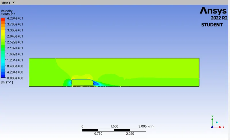
Please refer the below photo for the Velocity countor
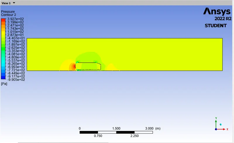
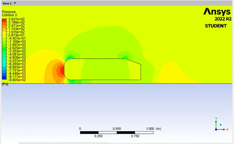
Please refer the below photo for the Pressure countor
Please refer the below photo for the Velocity vector
3) Following results are obtained for the fine mesh
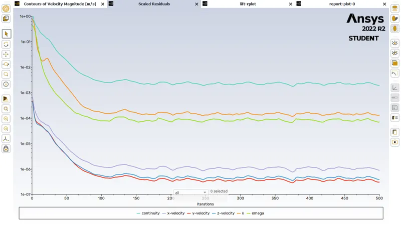
Please refer the below photo for the Residuals plot
Please refer the below photo for the drag plot
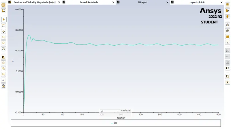
Please refer the below photo for the lift plot
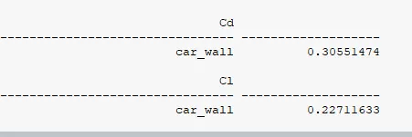
Please refer the below photo for the drag and lift coefficent value obtained
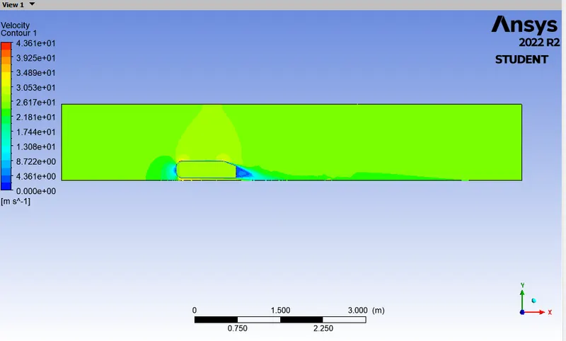
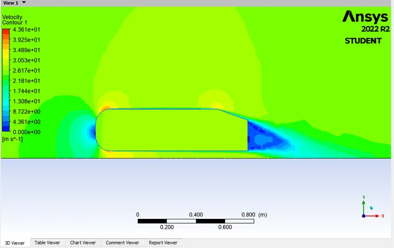
Please refer the below photo for the Velocity countor
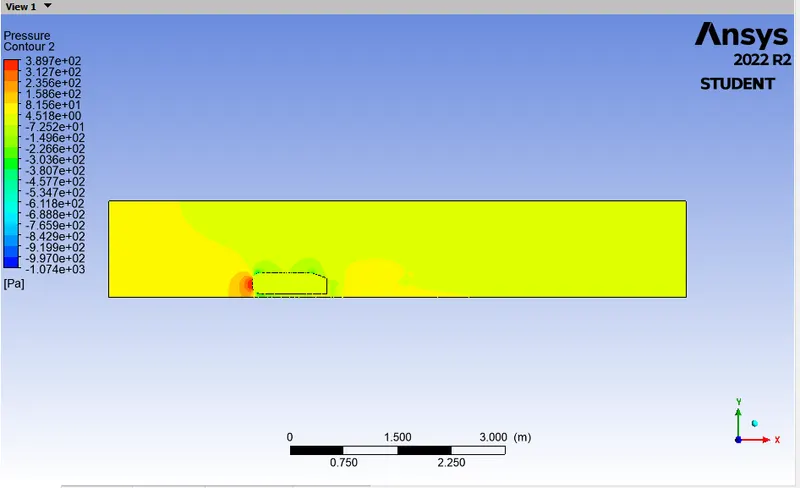
Please refer the below photo for the Pressure countor
Please refer the below photo for the Velocity vector
Conclusion:
There is a variation of pressure across the Ahmed body. The pressure in front of the body is positive because that's the location where the flow first comes in contact with the body and comes to rest. At the corner, the flow accelerates, thereby decreasing the pressure.
The reason behind negative pressure in the wake region is due to flow separation, recirculating flow. It's a phenomenon that generally happens as the air moving past the body isn't able to pass through the immediate backside of the body creating a region, where there is no movement of air and thereby creating a pressure gradient.
As the wake flow is the main contributor to the drag force(pressure drag), the point of separation is an important aspect of the flow. The more attached the flow is to the body the recirculation zone will be smaller and hence reduce the adverse effect of pressure drag, improving the fuel efficiency of the body.