Week 5 - Rayleigh Taylor Instability

AIM: To understand the Rayleigh Taylor Instability

INTRODUCTION:

• What is Rayleigh taylor instability?

The RT-instability is an instability that occurs at the intersection of two or more fluids with different densities. Whenever a heavier fluid (a fluid with greater density) is kept over a lighter fluid (lower density), due to gravity the the heavier fluid flows downwards, displacing the lighter fluid which gives to the deformation of the interference layer and mixing occurs.

Examples: Pouring milk/cream in a coffee mug, supernova explosions in which expanding core gas is accelerated into denser shell gas etc.

• What are some practical CFD models that have been based on the mathematical analysis of Rayleigh Taylor waves? In your own words, explain how these mathematical models have been adapted for CFD calculations.

• Kevin helmholtz instability

This instability can occur when there is velocity shear in a continous fluid, or where there is a velocity difference across the interface between two fluids.

• Richtmeyer-Meshkow Instability

This instability occurs when a shock wave interacts with an interface separating two different fluids or in other words when two fluids of different densities are impulsively accelerated.

• Plateau-Rayleigh Instability

This instability explains why and how a falling stream of fluid breaks up into smaller packets with the same volume but different or small surface area. It is often called as Rayleigh Instability. The driving force of this instablity is that the liquids by virtue of their surface tensions, tend to minimize their surface area.

• What is multiphase flow?

Multiphase flow is the flow of material with different phases like liquid-gas, gas-solid etc. OR the flow of different materials in the same phase.

• What is Volume of fluids method?

The volume of fluids method is a surface tracking method which is used to find the interference between two or more immiscible fluids. VOF measures the volume fraction of the liquid to determine the dominance of the respected fluid on a cell.
`alpha` is used to calculate the volume fraction.

`0<=alpha<=1`

Where `alpha` denotes the domination of a fluid. We will understand this with the experiment ahead.

SOLVING:

Designing the geometry:

• We will create the geometry in ANSYS Spaceclaim.
• We need to create two rectangular plates for different phases.
• We will select the X-Y plane and create a rectangle of 20mm x 20mm dimensions.

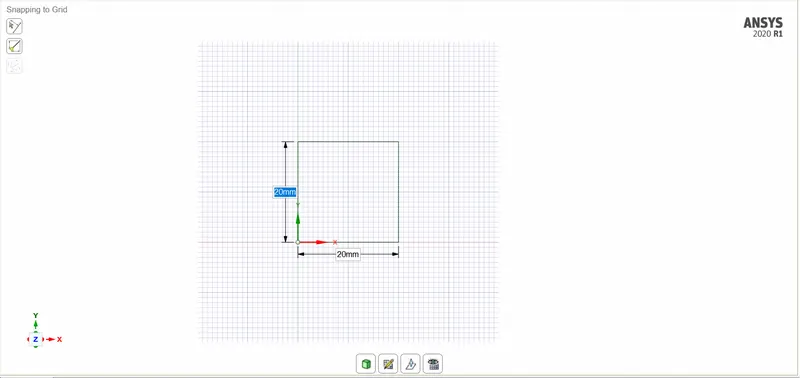
• We will use the pull feature to convert the sketch into 2D surface.

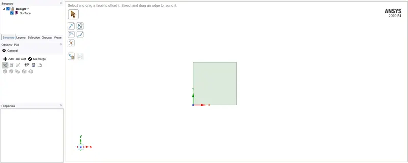
• After the surface has been created, we will name the surface to be air.

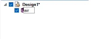
• Next we will create two components air and water.
• After that, selecting the water surface, we will create the same surface with same dimension.

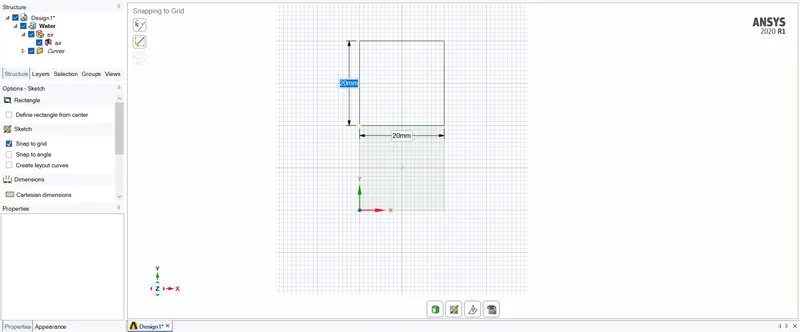
• Using the pull feature we will convert the sketch to a surface.

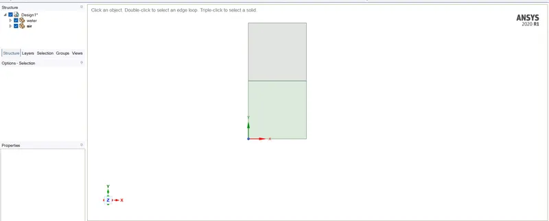
• We have created the geometry needed for the experiment. Now, we will move to the workbench tab and click on share.

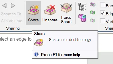
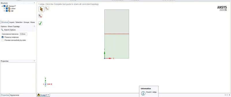
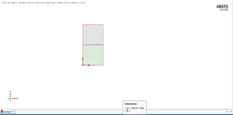
• Once we have shared both the surfaces, we have completed the geometry and can exit spaceclaim.
• We will now go to the mesh and create a mesh as mentioned in the question.

Meshing:

Case -1:

• We will create a base mesh of 0.5mm.

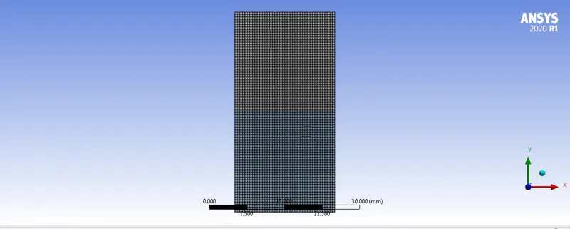
• Once the mesh has been created we will update it and will move to Fluent to provide the boundary conditions.

Providing boundary conditions:

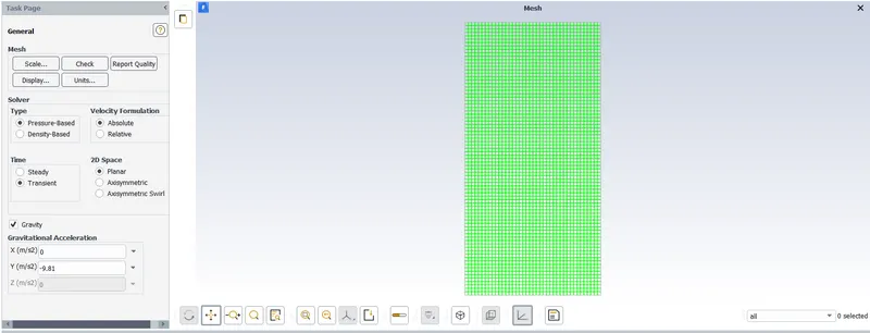
• For the experiment we will be using a pressure based solver. The simulation will be transient.
• We will also provide gravity at the y-axis.

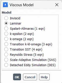
• We will select the model to be Laminar.

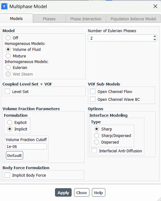
• In the multiphase section, we will select Volume of fluids (VOF) method and select implicit method for solving.

• Now we will use two materials. The lower section will be filled with air and the upper section will be filled with water. Thus, we need to make sure we have the specified materials.

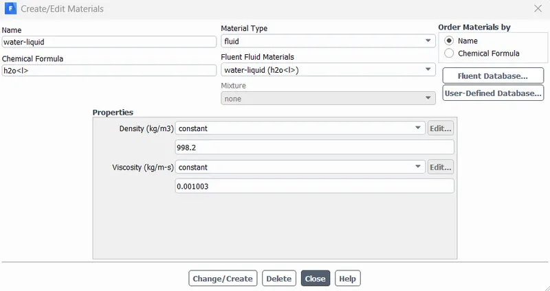
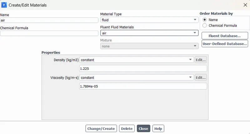
• After the materials have been specified, we will select the phases and select appropriate material for the respective phase.

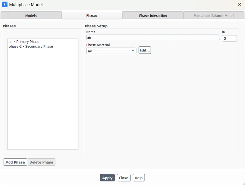
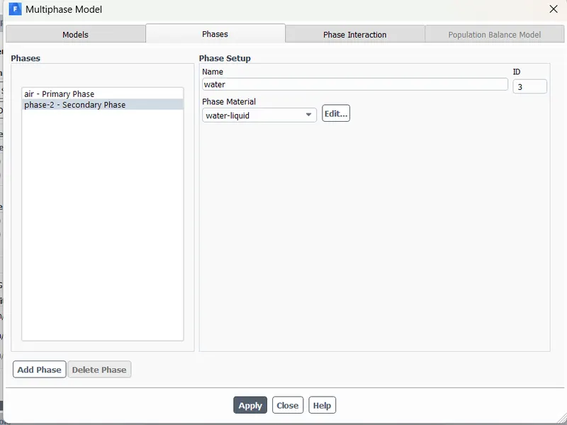
• Once the phases have been assigned, we will go to the patch section and provide the value of alpha.
• Before that we need to initialise the problem.
• We will give the value of `alpha` to be 1 for water at the water surface and zero at the air surface symbolising zero cells filled with water at the air surface.

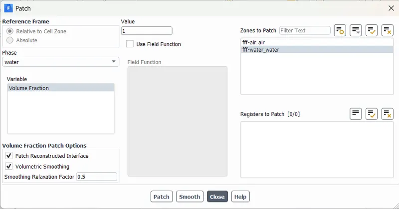
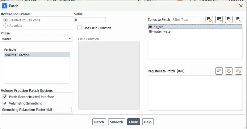
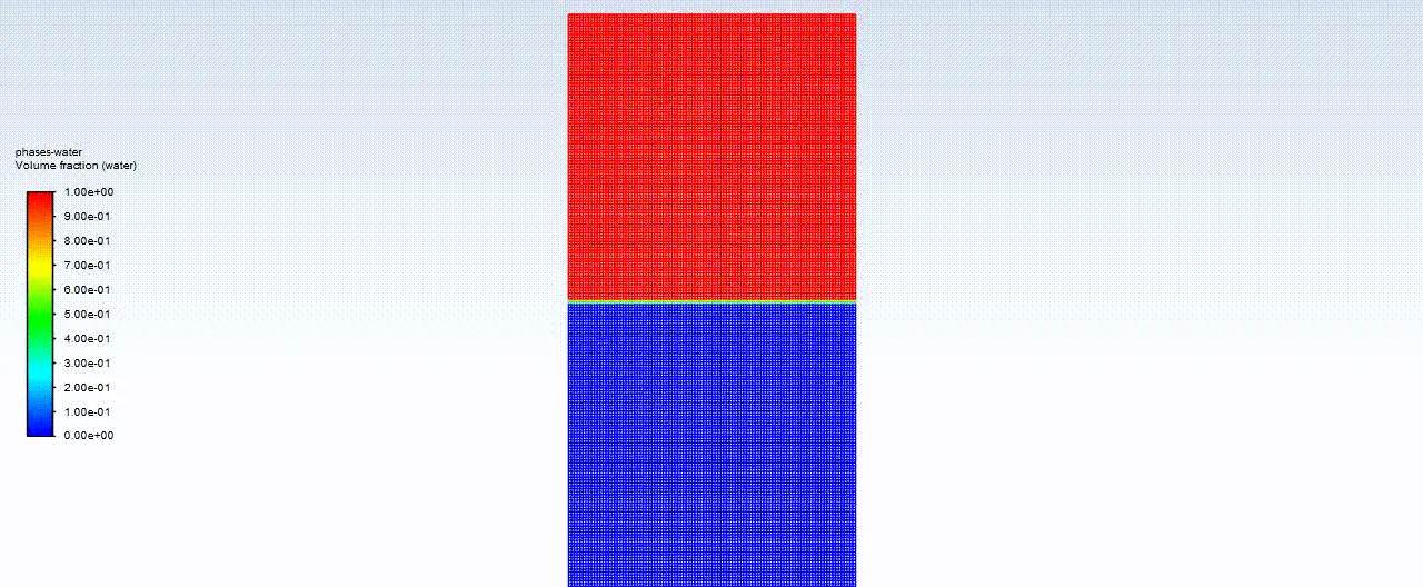
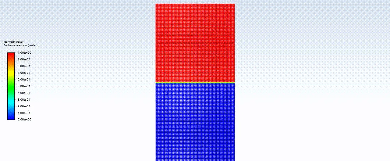
• To check whether the boundary conditions provided are correct or not. We can go create a contour showing the phases.

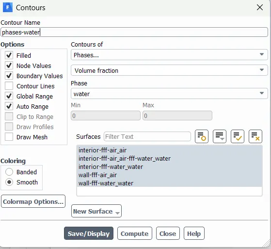
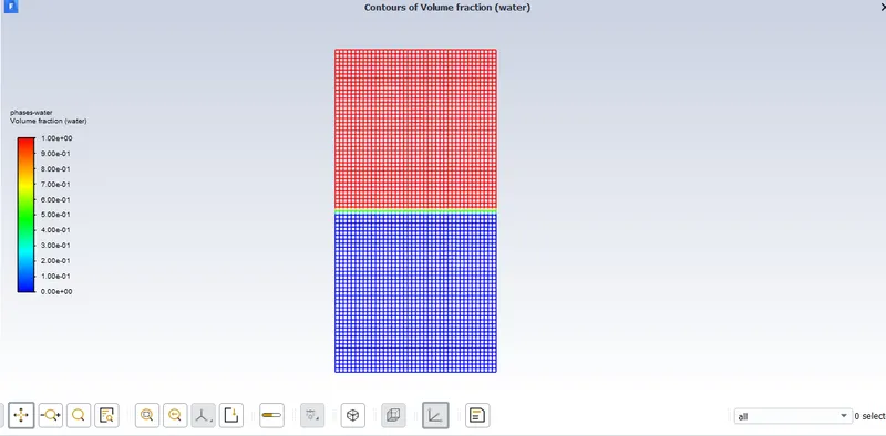
• From the plot, it is clear that the volume fractoin given is accurate.
• We can go forward and calculate by providing the time-step size and no. of time steps.
• I have to run the calculation for 2 seconds thus I can use the time step size to be 0.01 and number of time steps to be 200.

RESULTS FROM BASE MESH:

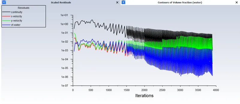
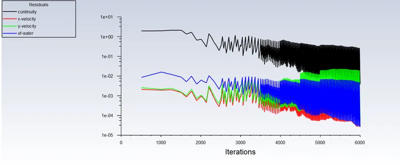
• Scaled residuals:

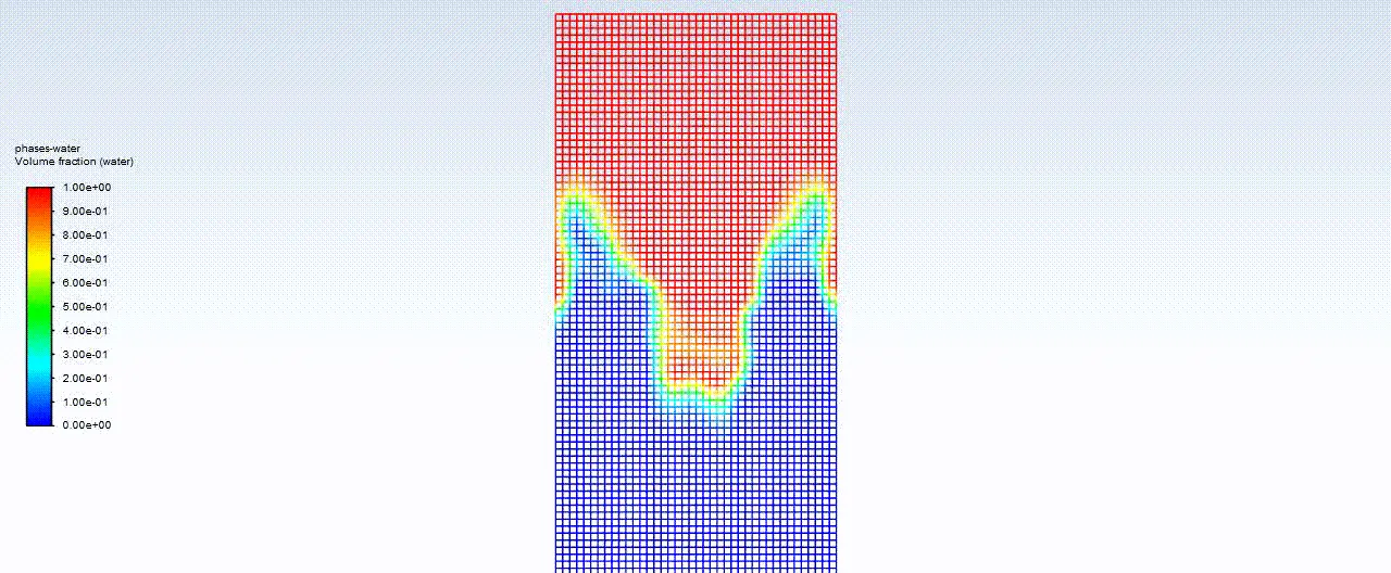
• Animation of RT-instability.

Case- 2: Refined mesh

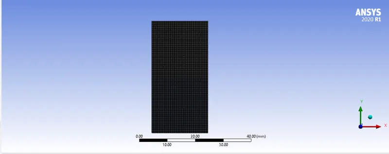
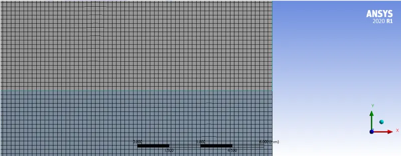
• For the following case we will refine the mesh to observe the variation in results. We will be using a mesh size of 0.1mm.

• We will now move to the fluent section to provide the boundary conditions. The boundary conditions to be provided are the same as before.

RESULTS:

• Scaled residuals

• Animation of RT-instability:

CONCLUSION:

• As we refine the mesh, we can better evaluate the instability taking place due to mixing of two fluids with different densities.
• As we reduce the mesh length, the time taken to evaluate the results increases i.e., increased computational time.

We are using a transient approach to solve the RT-instability problem because we need to capture instability which are varying with respect to time thus using a steady state approach might now be suitable.

Case 3: User specified material.

• In this case, the material to be used has a density of 400 kg/m³ and viscosity of 0.001 kg/m-s. We will be using the refined mesh.

Input material properties:

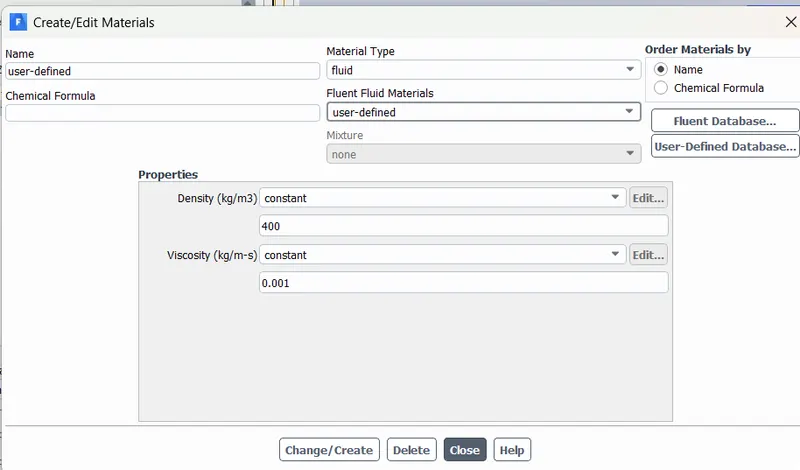
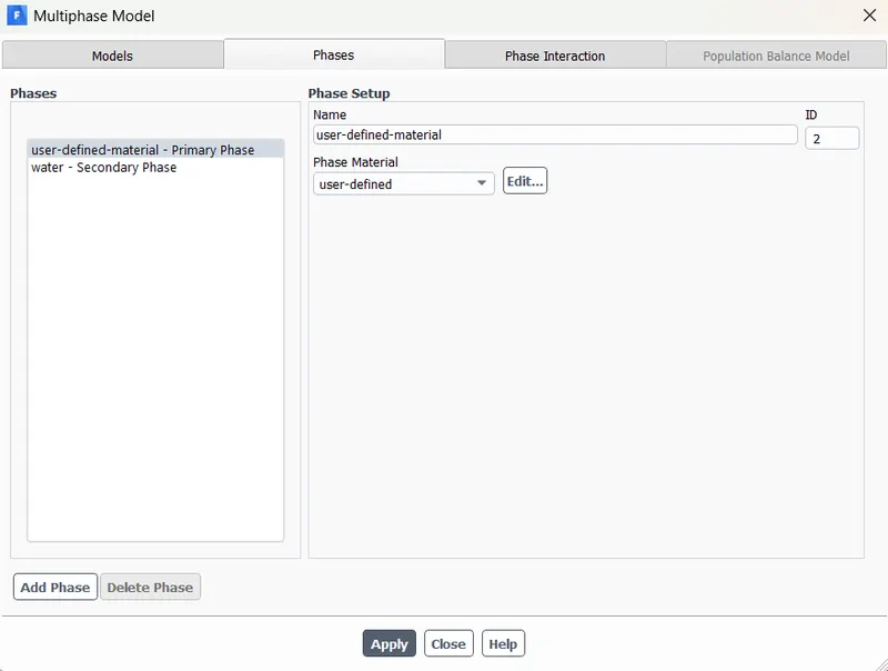
• Once we have added the materail details, we can move forward and perform initialisation.
• To check whether we have done the phase selection correctly, we can plot the phase contour.

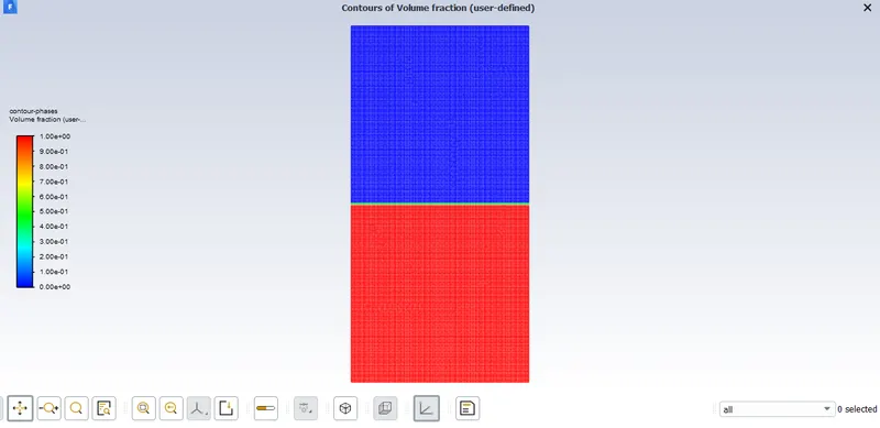
RESULTS:

• RT-animation:

Define the Atwood Number. Find out the Atwood number for both the cases and explain how the variation in Atwood number in the above two cases affects the behavior of the instability.

• Atwood Number:
  • Atwood number is a dimension-less number used to study hydrodynamic instabilities in density stratified flow.

Atwood number (A) = `(rho_1 - rho_2)/(rho_1+rho_2)`

where,

`rho_1` = density of heavier liquid.

`rho_2` = density of lighter liquid.

• For case - 2:
  • `rho_1` = density of water = 997 kg/m³
  • `rho_2` = density of air = 1.225 kg/m³

Atwood number for case - 2 is 0.997.

• For case-3:
  • `rho_1` = density of water = 997 kg/m³
  • `rho_2` = density of user defined material = 400 kg/m³.

Atwood number for case - 3 is 0.427.

OBSERVATION:

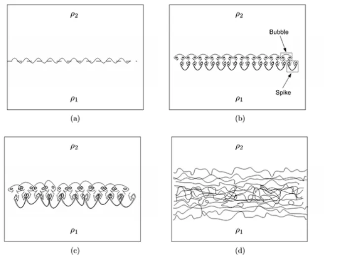
• The image shown below shows the steps involved in the formation of RT-instability.
• At first the disturbances are small when compared to their wavelength which then gets converted to mushroom shaped spikes and bubbles. These fluid structures mix together causing them to blend and mix with each other which then eventually develops into a mixing region.

CONCLUSION:

• The atwood number can predict the formation of these instabilities.
• For A close to 0, RT instability flows are more symmetric. For A close to 1, the much lighter fluid "below" the heavier fluid takes the form of larger bubble-like plumes which can also be observed in our case.
• We can see that for low atwood number i.e., case - 3, the bubbles and mushroob spikes formed are symmetrical and then they mix together whereas for large atwood number i.e., case - 2, the mushroom heads and bubbles formed are less symmetrical and form at an accelerated pace.