Week 1- Mixing Tee

Aim: Simulation of a Mixing Tee using ANSYS Fluent.

Introduction and theory:

1. What is a Mixing Tee?
   • A mixing tee is a pipe like geometry which has two inlets provided within it and an outlet where the flowing entity is measured.
2. Where is it used?
   • A mixing tee is used when you want to mix two different fluids with different temperature to get a fluid at the output with the desired temperature.
   • E.x: Lets say you need to reduce the temperature of a room but the cooling unit you have has a fixed coolant temperature of -10°C. Now, that is a very low temperature for a person to feel comfortable within a room. In order to get the desired temperature within the room, we will use a mixing tee. The mixing tee will mix the coolant with the fluid at a different temperature and on the basis of their mixture we will be able to generate a fluid of the desired temperature.

Overview of the study:

• In this study, we will conduct two experiments which will contain two different Mixing tee model of varying length.
• We will be studying two different cases:
  • Case 1
    • Short mixing tee with a hot inlet velocity of 3m/s.
    • Momentum ratio of 2, 4.
  • Case 2
    • Long mixing tee with a hot inlet velocity of 3m/s.
    • Momentum ratio of 2, 4.
• From the experiment we will try and find out how:
  • Change in geometry effects output temperature.
  • Change in velocity effects individual cases.
  • The best geometry with the best boundary conditions for mixing.
• For the first case, we will solve the problem by using K-epsilon and K-omega model and figure out which model is more suitable for our problem.

Procedure:

• Geometry cleanup:
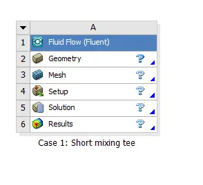
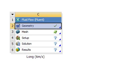
  • We will first open ANSYS Workbench and select the Fluent module for our experiment.
    • 
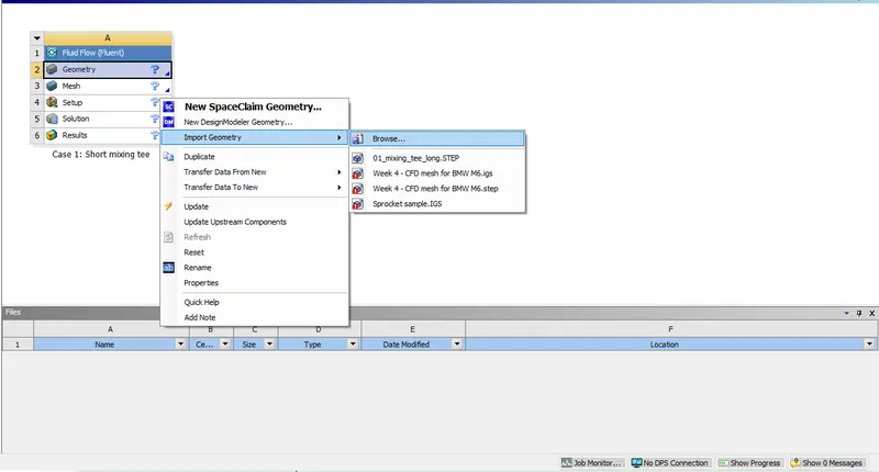
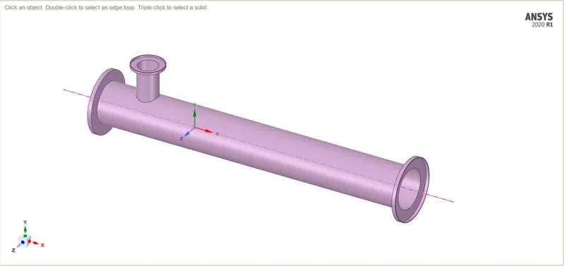
  • We will import the model into the geometry section and open SPACECLAIM.
    • 
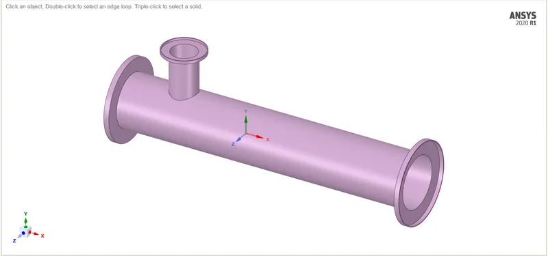
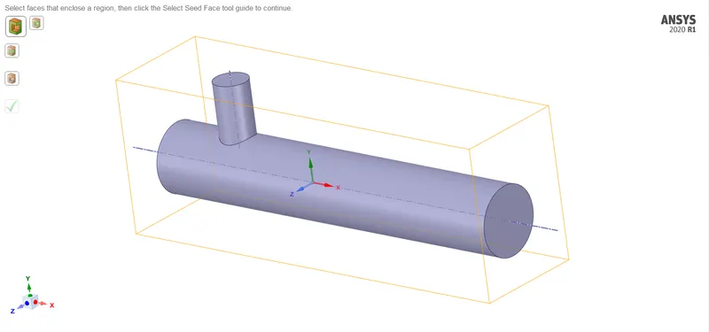
  • The spaceclaim window looks like the image given below.
    • 
  • For the experiment we are about the perform, we do not need extra features like the thickness given at the inlet and outlet sections. We will select the internal volume of the geometry and perform out analysis on it.
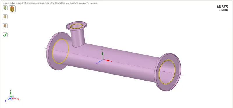
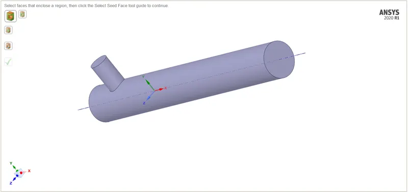
  • To accurately select the internal volume, we will use the VOLUME EXTRACT feature.
• Note: The volume extraction feature is used to extract the internal volume of the geometry. With this feature, we will be able to create a single solid body representing the volume for the model.
  
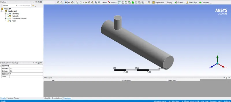
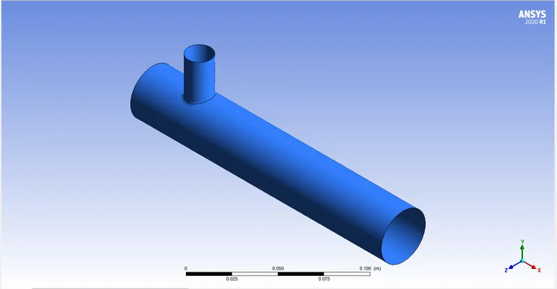
  • The required volume for the geometry looks like the image given below.
    • 
    • 
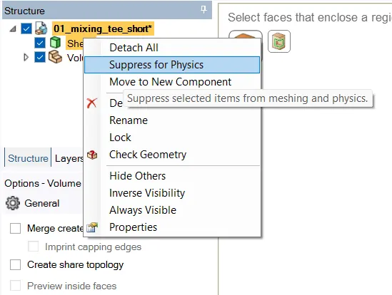
  • After the volume has been created we need to supress the orginial model for physics which will supress the orignial model meshing we will perform in the mesh section.
    • 
• Meshing:
  • After this, we can close Spaceclaim and open the meshing window.
    • 
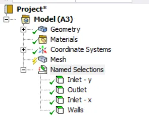
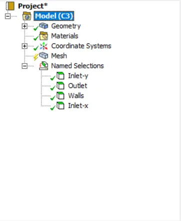
  • Before we mesh, we will name the boundaries using the Named selection feature.
  • We have to name four surfaces as
    • Inlet - x: The inlet in x direction.
    • Inlet - y: The inlet in y direction.
    • Outlet: The outet of the model.
    • Walls: The walls of the model.
  • After naming the required boundaries, you can view the names in the tree structure on the left side of the screen.
    • 
  • The next step is to generate the mesh.
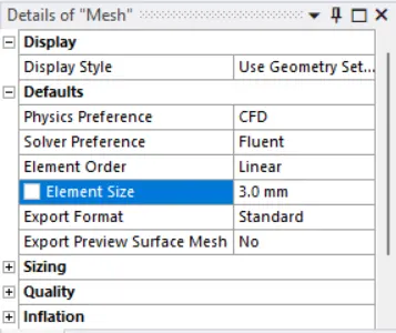
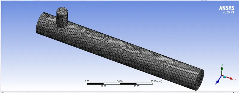
  • We would provide a fine mesh by giving the mesh length as 3mm.
    • 
    • 
  • After the mesh has been generated, we can close the meshing module and open Fluent launcher.

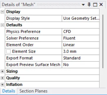
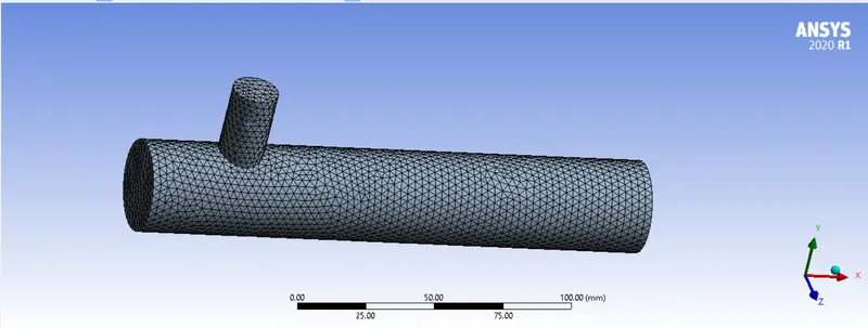
Note: During the first case, we will analyse which model is more suitable for our experiment and with the next case we will use the better model.

• Case 1 (a):
  • While solving for case 1, we will use use both K-epsilon and K-Omega SST model to analyse the results.
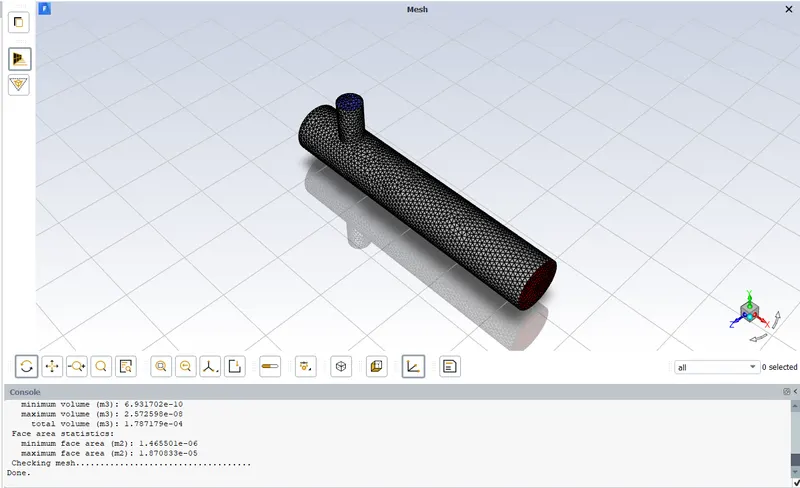
  • Once we have loaded the model in Fluent launcher we will check the mesh using Mesh check.
  • After the mesh has been checked, we can move forward and select the model according to our problem.
  • First, we will select K-omega model and input the necessary boundary conditions.
  • K-Omega SST:
    • We will turn on the energy equation and from the viscous model, we will select K-omega SST.
      
      • 
    • After this, we will select the material to be air.
    • We will check whether the cell zone condition is fluid and check for the input of fluid to be air.
      • 
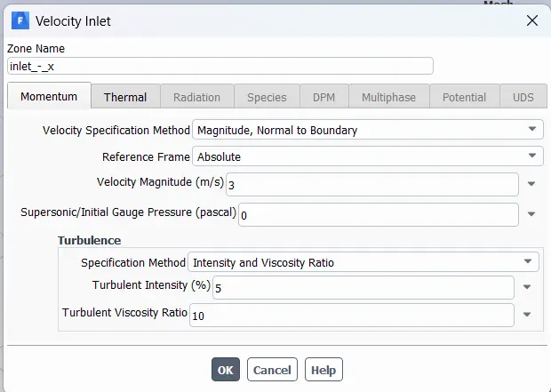
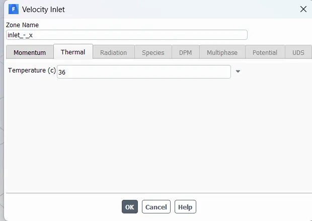
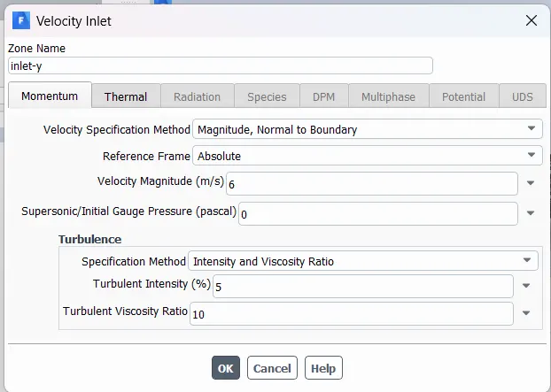
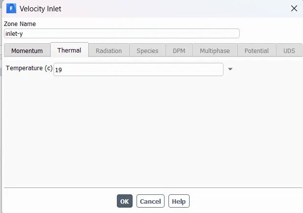
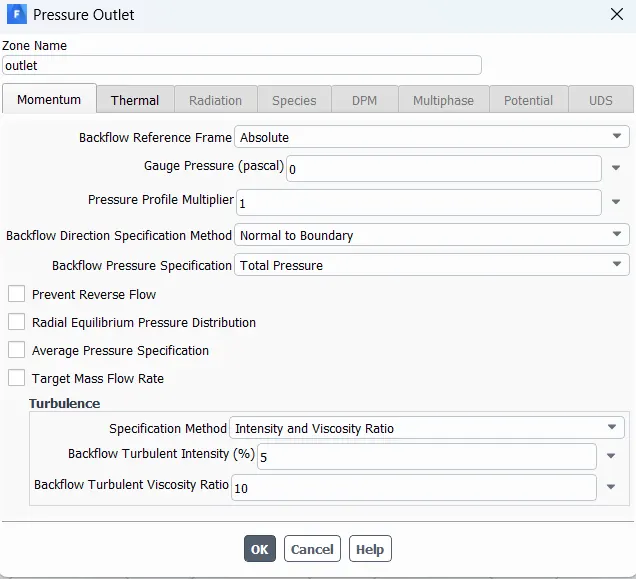
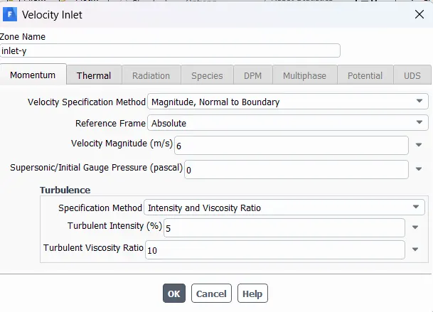
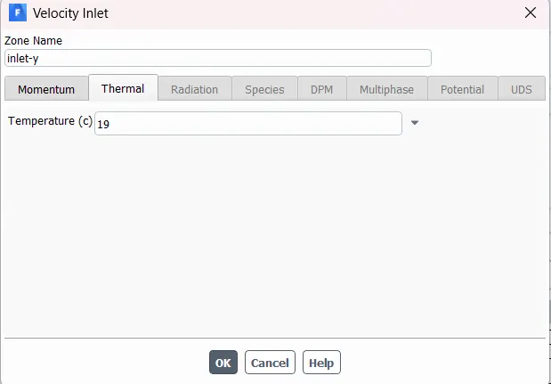
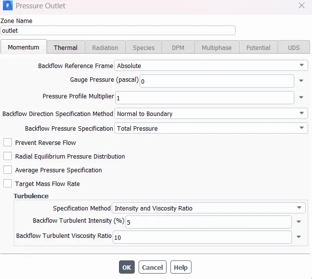
    • We will go to the boundaries and give the necessary boundary conditions.
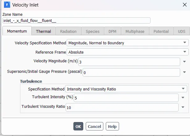
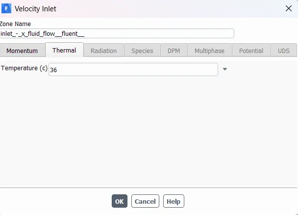
    • In terms of case-1(a), the boundary conditions are:
      • Inlet - x:
        • Velocity: 6m/s.
        • Temperature: 36⁰C.
      • Inlet - y:
        • Velocity: 3m/s.
        • Temperature: 19⁰C.
      • Outlet:
        • Gauge pressure: 0 pa.
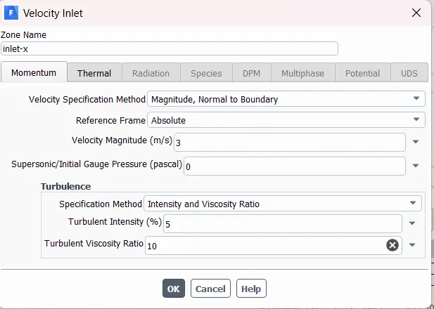
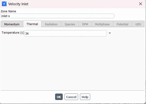
    • The following images show the boundary conditions:
      • 
      • 
      • 
      • 
      • 
  • We will generate two reports:
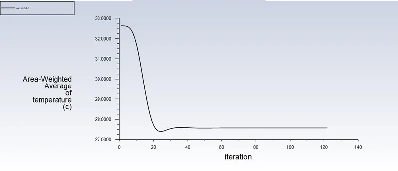
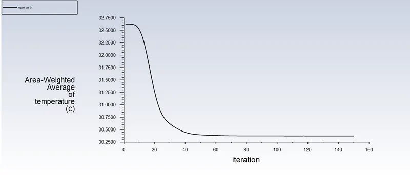
    • The area weighted average of temperature at outlet.
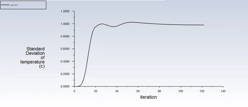
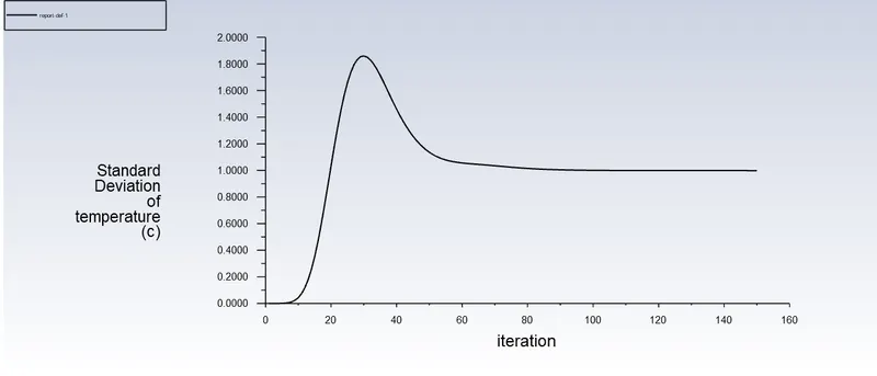
    • Standard deviation of temperature at outlet.
  • We will initialize the model and perform a total of 150 iterations.
  • After the calculations have been performed we can go to the results tab and check the results of the experiment we performed.
• Results of K-Omega SST model:
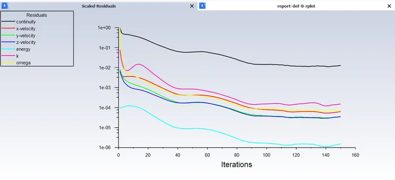
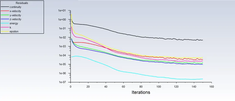
  • Residual plot:
    • 
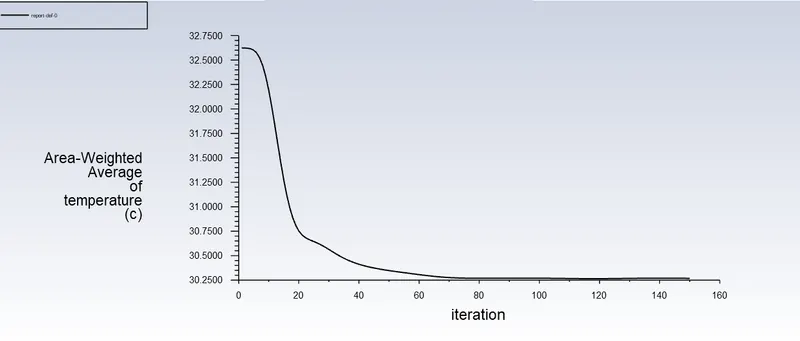
  • Area weighted average of temperature at outlet:
    • 
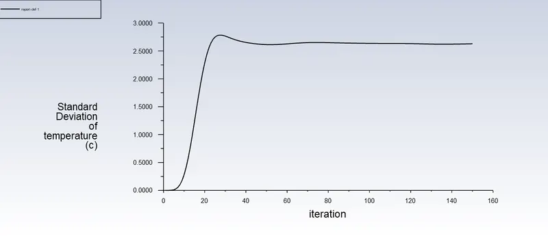
  • Standard deviation of temperature:
    • 
  • Temperature variation:
    • 
  • Velocity variation:
    • 
  • Now we will do the simulation again by chaning the model to k-epsilon.
  • K-epsilon:
    • We will use the same boundary conditions but change the viscous model to K-epsilon and run the model for 150 iterations.
• Results of K-epsilon model:
  • Residual plot:
    • 
  • Area weighted average temperature at outlet:
    • 
  • Standard deviation of temperature at outlet:
    • 
  • Temperature variation:
    • 
  • Velocity variation:
    • 
  • Temperature plot:
    • 
  • Velocity plot:
    • 
• Observation:
  • From the observation of the results obtained from both the models we can see that the deviation in terms of output is not very large value. However, from the K-omega model we are able to see that the model is more suited for observing flow near the walls of the geometry as well. From the contours of velocity, it is evident that K-epsilon model was capturing the finer details of flow within the inner regions of the mixing tee whereas the K-Omega model is not being able to do that. Since, the main objective of the experiment is to study the flow within the mixing tee we will choose k-epsilon model as it is more suited for internal flow.
  • Thus, for further calculation we will continue with the K-epsilon model.
• Since the analysis for case - 1 was done, we can move to the next condition for case - 1
• Case - 1 (b):
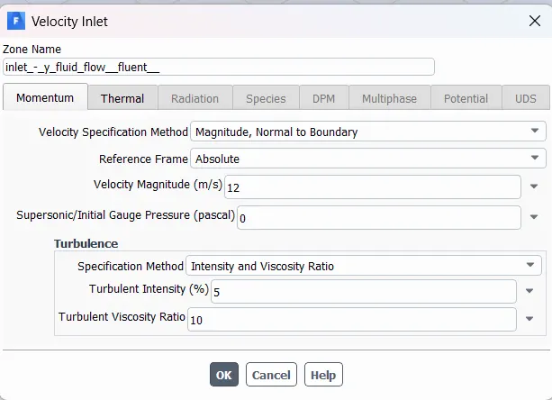
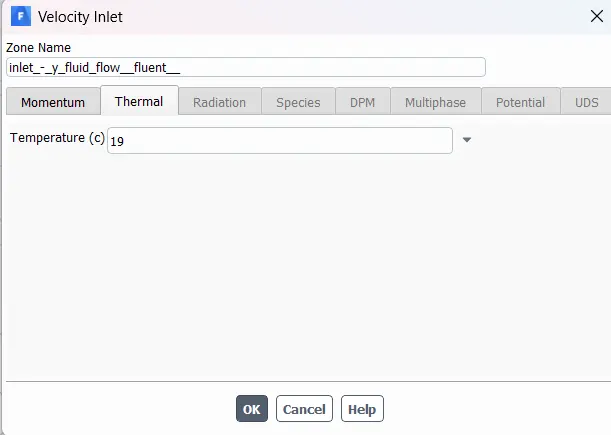
  • In terms of case-1 (b), the boundary conditions are:
    • Inlet - x:
      • Velocity: 12m/s.
      • Temperature: 36⁰C.
    • Inlet - y:
      • Velocity: 3m/s.
      • Temperature: 19⁰C.
    • Outlet:
      • Gauge pressure: 0 pa.
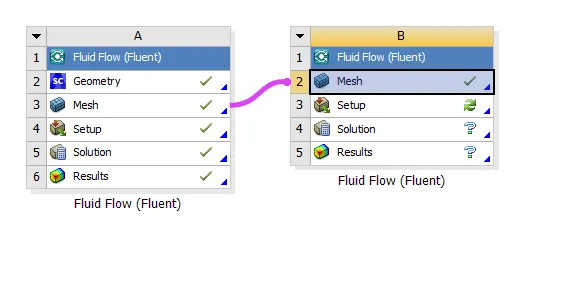
  • We can select and drag one more fluent solver as shown in the image below to save us time from re-meshing the entire geometry.
    • 
  • We can open the fluent solver and start setting up the necessary models, material, boundary conditions etc.
  • Once the model has been loaded in the Fluent we can start with checking the mesh.
    • 
  • We will be using a pressure based solver.
  • After checking the mesh, we can select the model as K-epsilon and turn on the energy equation.
    • 
  • We need to make sure the material selected is air and the cellzone condition specifies it to be fluid where the fluid is air.
  • Now we can setup the boundary conditions.
    • 
    • 
    • 
    • 
• Results (plots) :
  
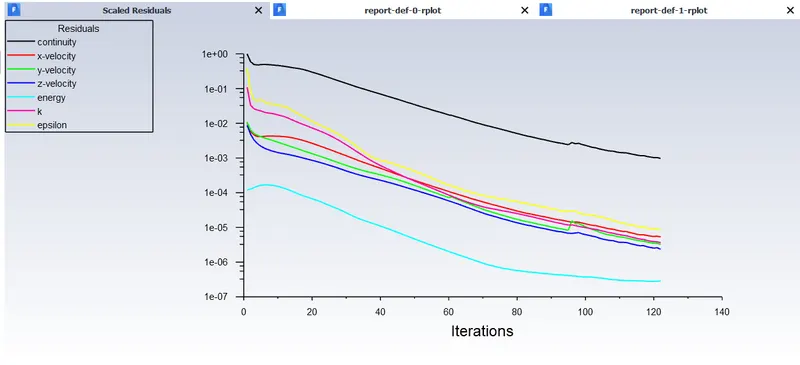
  • Scaled residuals:
    • 
  • Area weightage average of temperature at outlet:
    • 
  • Standard deviation of temperature at outlet:
    • 
  • Now we can move the Result section to view the temperature and velocity variation throughout the model.
  • We need to set the exact plane and view to make sure we view the result properly.
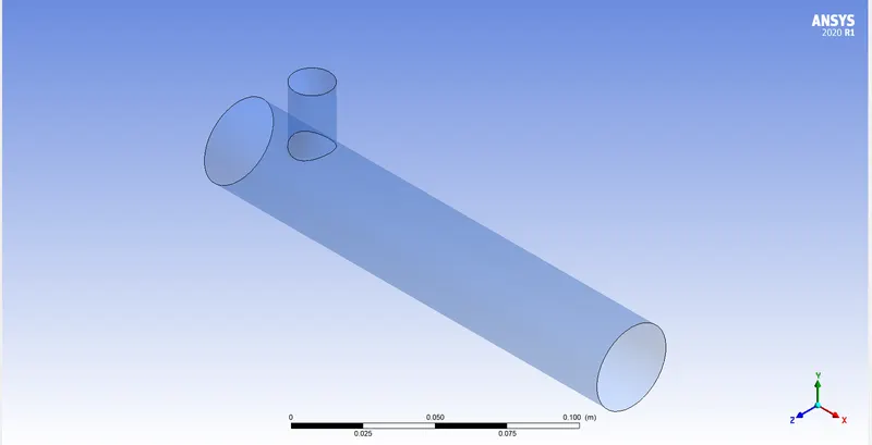
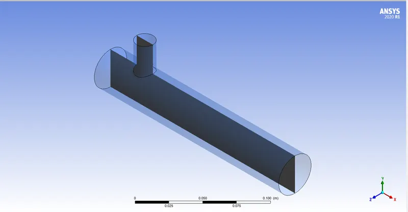
  • We will create transperency between the walls of the model to examine the temperature and velocity contour well.
    • 
    • 
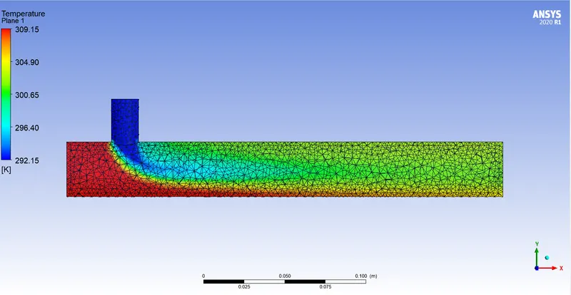
  • We will generate a plane in the XY plane exactly at the middle of the geometry to display the temperature and velocity contour.
    • 
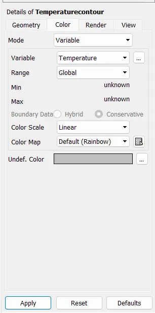
  • We can colour the plane using the variable temperature.
    • 
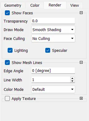
  • We can also activate the mesh lines to view the contour smoothly.
    • 
  • We can now examine the plots that has been generated.
• Results (contour and plot):
  • Temperature contour:
    • 
    • 
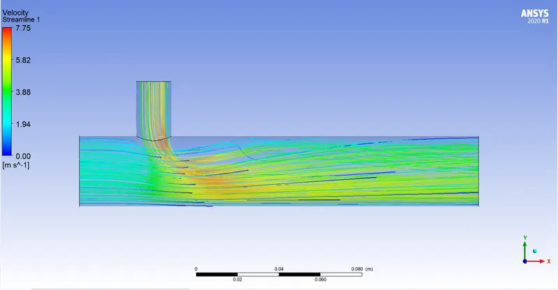
  • Velocity contour:
    • 
    • 
  • Since case 1 has been solved completly, we can move to case 2.
• Case 2 (a):
  • We will select the fluent module from ANSYS and drag it to the prjoect schematic window.
  • After that we can import the geometry into Geometry and open spaceclaim to select the internal volume that we need for the analysis.
    • 
    • 
  • Using the volume extract feature, we will extract the volume that we require to perform the analysis.
    • 
  • We will supress the previous geometry for all meshing and physics.
  • After the volume has been extracted, we can move to the meshing portion.
• Meshing:
  • The first thing to do while we are in the meshing window is to create Names selections.
    • 
  • Once we have created the names selection, we can set the mesh length to be 3mm.
    
    • 
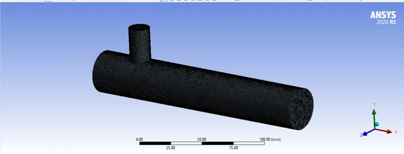
  • Once the mesh has been created it looks like the image given below.
    • 
  • After the mesh has been created, we will update the mesh and move to fluent window to solve for the given boundary conditions.
  • We need to check the mesh before we can start the process. We will use the check mesh option to check the quality of the mesh.
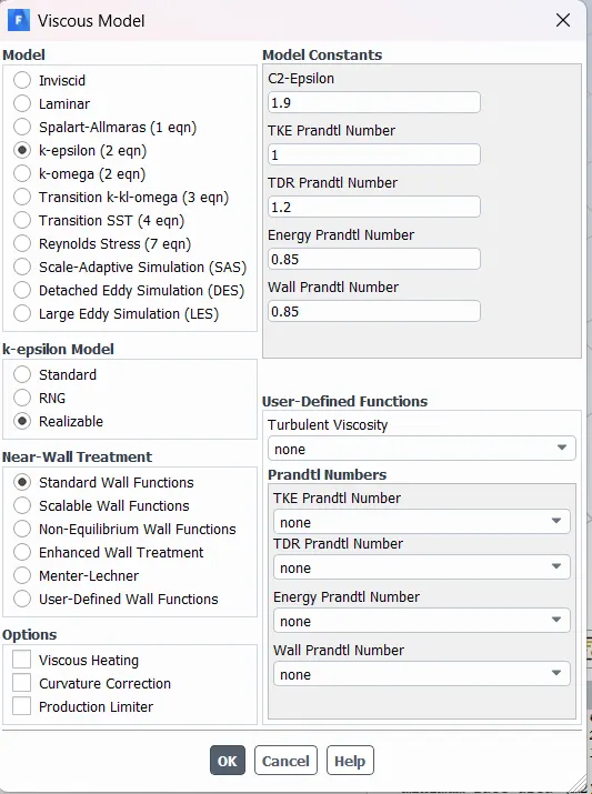
  • After the mesh has been checked, we can go to the Physics tab and turn on the Energy equation and select the model as K-epsilon with realizable standard wall function.
  • We can then check for the material to be Air and the cell zone condition to be fluid where the material to be used be air.
  • After that we can set our boundary conditions
    • Inlet - x:
      • Velocity: 6m/s.
      • Temperature: 36⁰C.
    • Inlet - y:
      • Velocity: 3m/s.
      • Temperature: 19⁰C.
    • Outlet:
      • Gauge pressure: 0 pa.
  • We will now input the boundary conditions according to our requirements.
    • 
    • 
    • 
    • 
    • 
  • Once the boundary conditions have been set we can move forward with the calculation.
  • Before calculating, we need to generate two seperate plots:
    • Area weighted average of temperature at outlet.
    • Standard deviation of temperature at outlet.
  • We will then initialise the problem and perform 150 iterations.
• Results (Plots):
  • Scaled residuals:
    • 
  • Area weighted average of temperature at outlet:
    • 
  • Standard deviation of temperature at outlet:
    • 
• We can now move on to the result section to view the temperature and velocity contour.
• We will create a plane in the xy plane as we made before to view the temperature and velocity contours.
• Results (Contour):
  • Temperature contour:
    • 
    • 
  • Velocity contour:
    • 
    • 
• Case 2 (b):
  • In terms of case-1 (b), the boundary conditions are:
    • Inlet - x:
      • Velocity: 12m/s.
      • Temperature: 36⁰C.
    • Inlet - y:
      • Velocity: 3m/s.
      • Temperature: 19⁰C.
    • Outlet:
      • Gauge pressure: 0 pa.
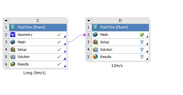
  • We do not need to recreate the entire mesh, we can drag a fluent module and share the geometries and the mesh as shown below.
    • 
  • We can move to the setup section, open fluent and provide the required boundary conditions and generate the same plots that we generated for the above problems.
  • We will perform 150 iterations in total.
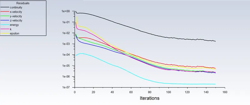
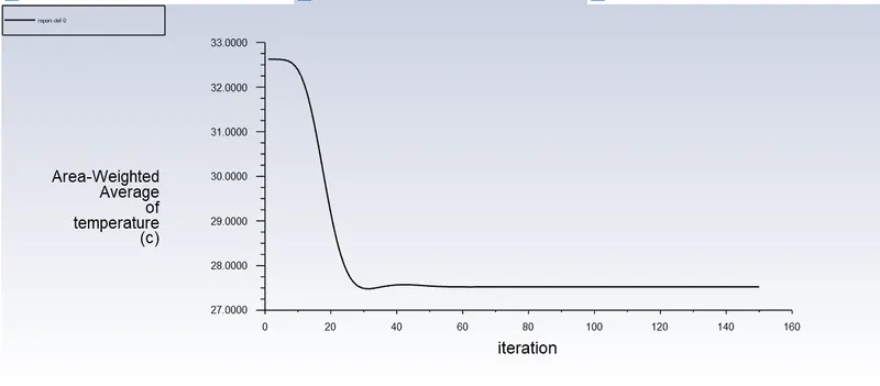
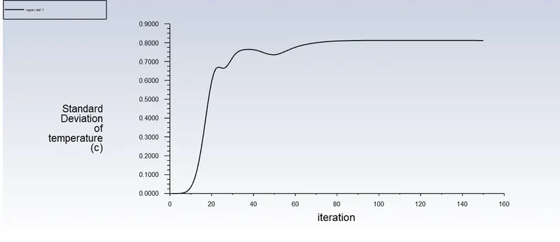
• Results (Plots):
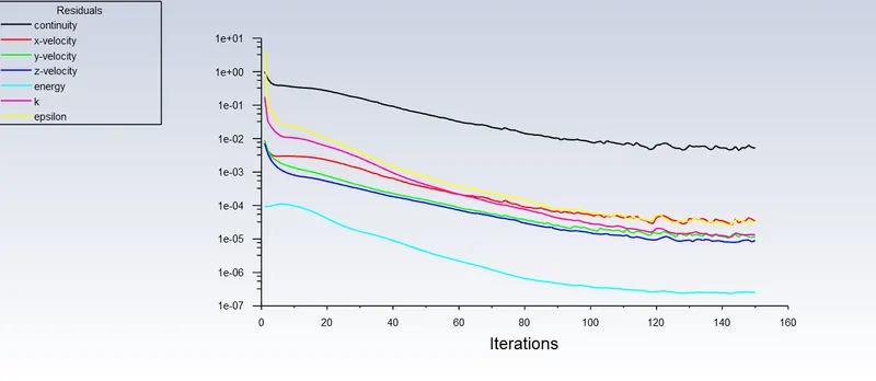
  • Scaled residuals:
    • 
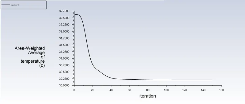
  • Area weighted average of temperature at outlet:
    • 
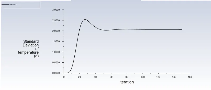
  • Standard deviation of temperature:
    • 
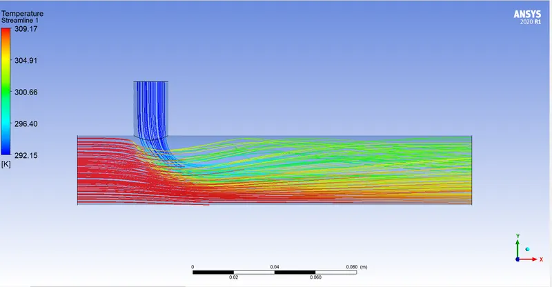
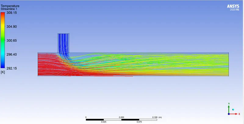
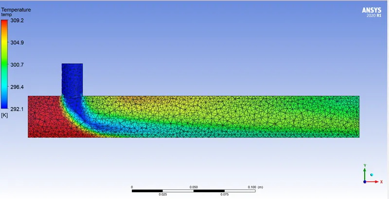
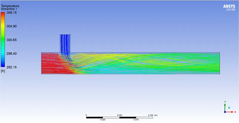
• Results (Contour and lines):
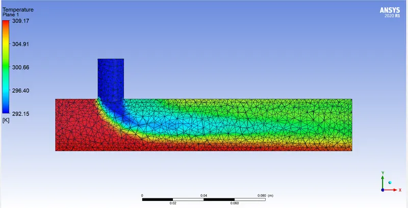
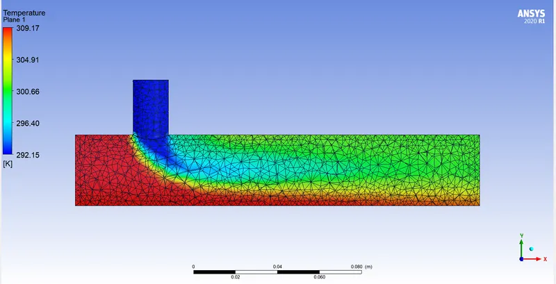
  • Temperature:
    • 
    • 
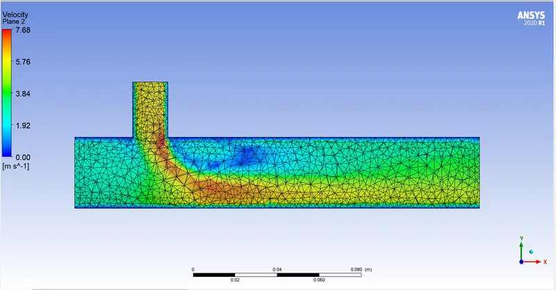
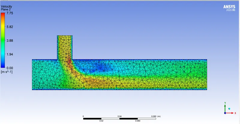
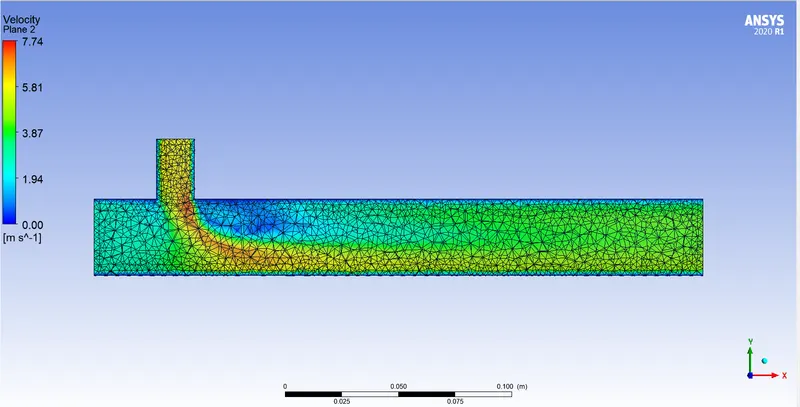
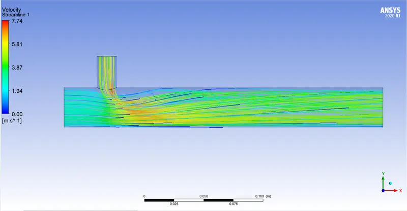
  • Velocity:
    • 
    • 

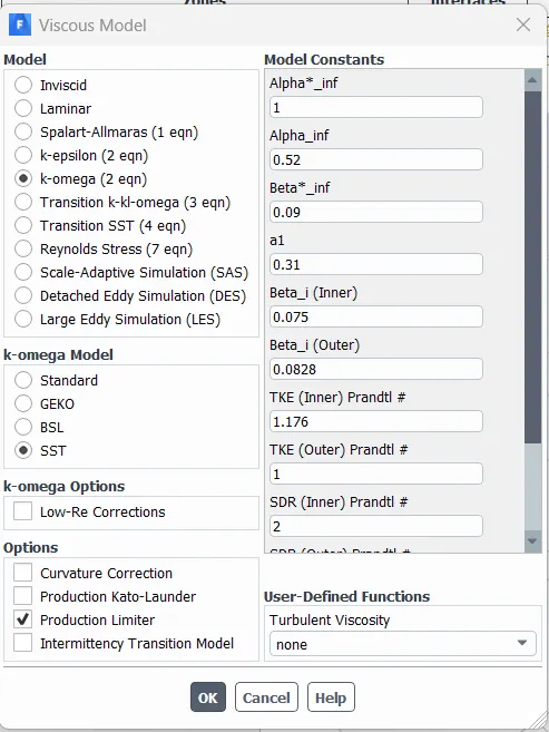
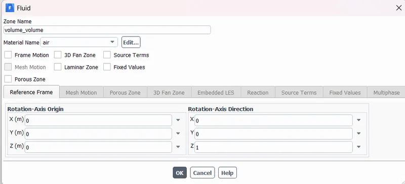
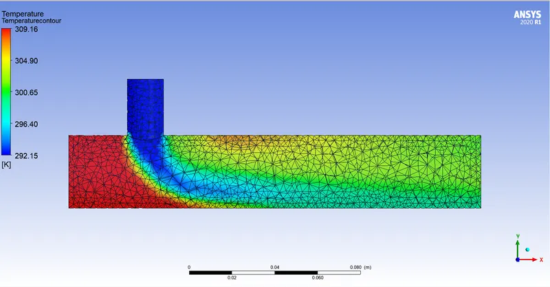
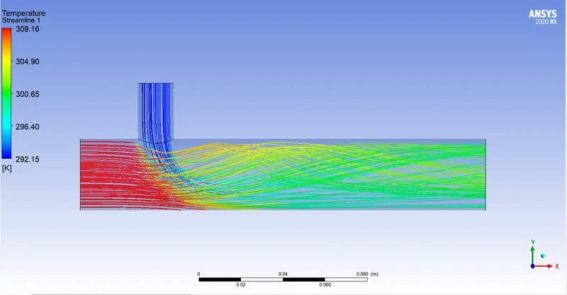
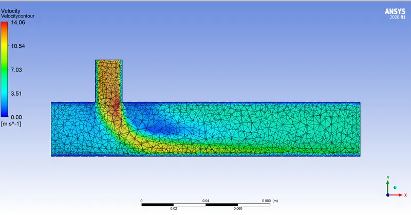
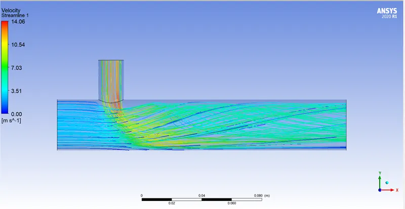
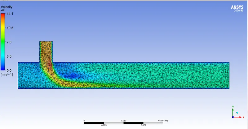
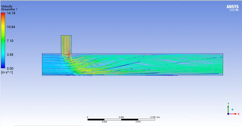
Observations:

• Condition	Case-1 (a)	Case-1 (b)	Case-2 (a)	Case-2 (b)
  Cell count	39,803	39,803	56,541	56,541
  Average outlet temperature	30.250 0C	27.75 0C	30.250 0C	27.25 0C
  Standard deviation	2.250	1.00	1.000	0.800

Mesh independent study:

• In this study, we will try to solve case 1 (a) with mesh of different lengths and calculate the effect mesh length has on results.
• The mesh length we are going to consider are 10mm, 5mm, 3mm, 1mm.
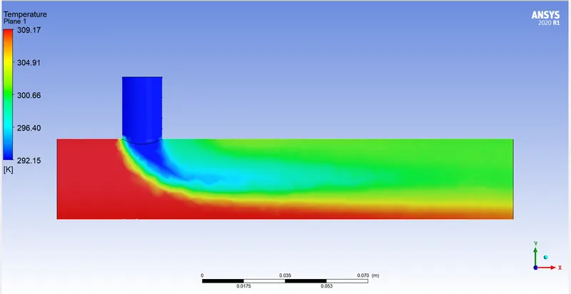
• 10mm mesh:
  • Mesh image:
    • 
  • Temperature contour:
    • 
    • 
• 5mm mesh:
  • Mesh image:
    • 
  • Temperature contour:
    • 
    • 
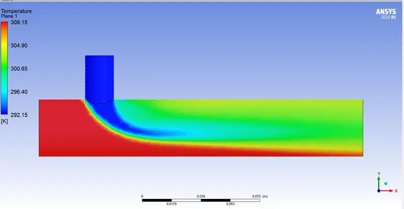
• 3mm mesh:
  • Mesh image:
    • 
  • Temperature contour:
    • 
    • 
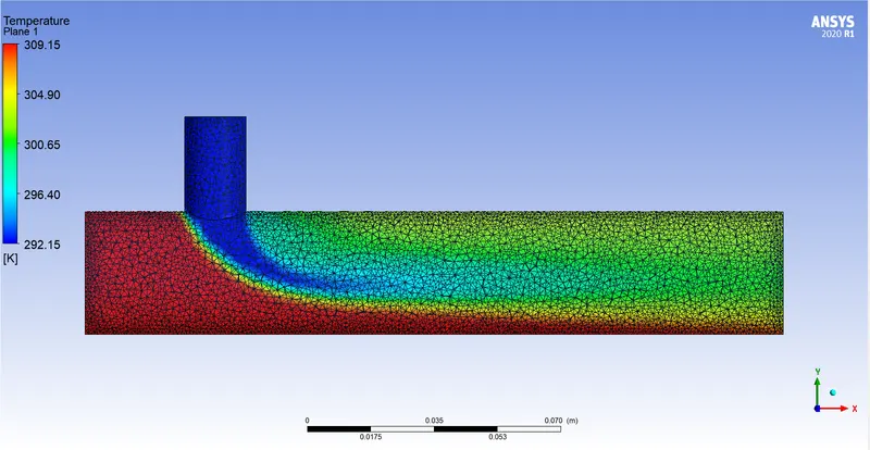
• 1mm mesh:
  • Mesh image:
    • 
  • Temperature contour:
    • 
    • 

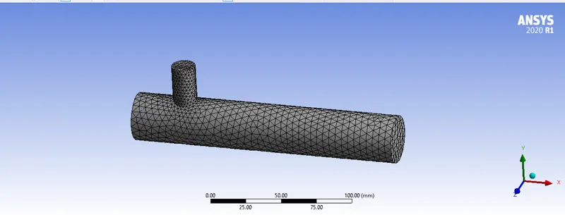
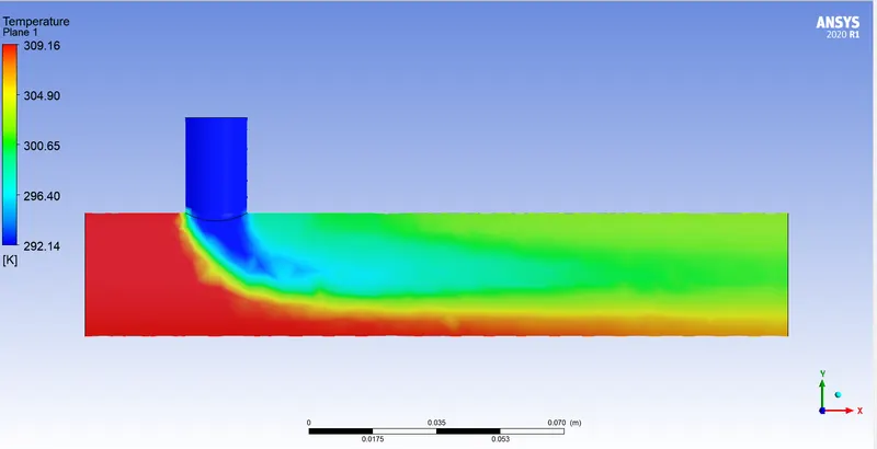
Result of independent mesh study:

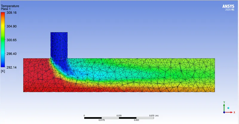
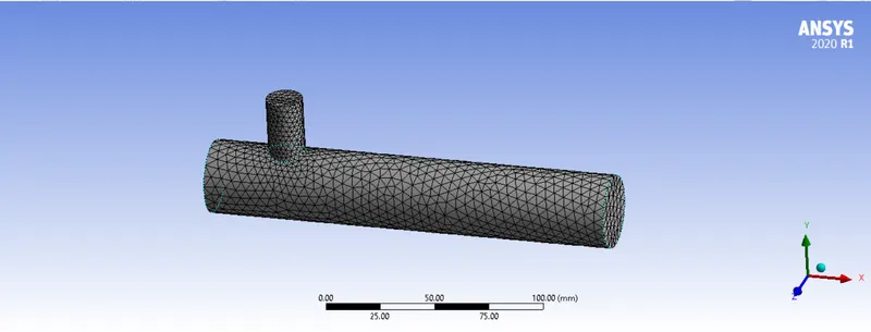
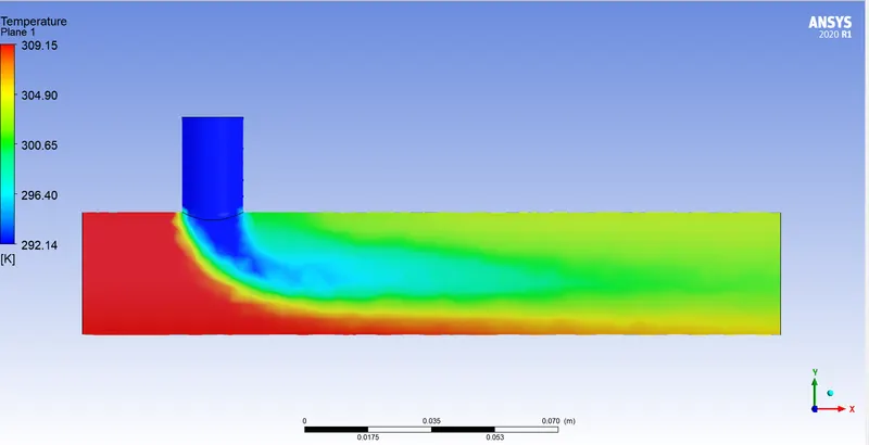
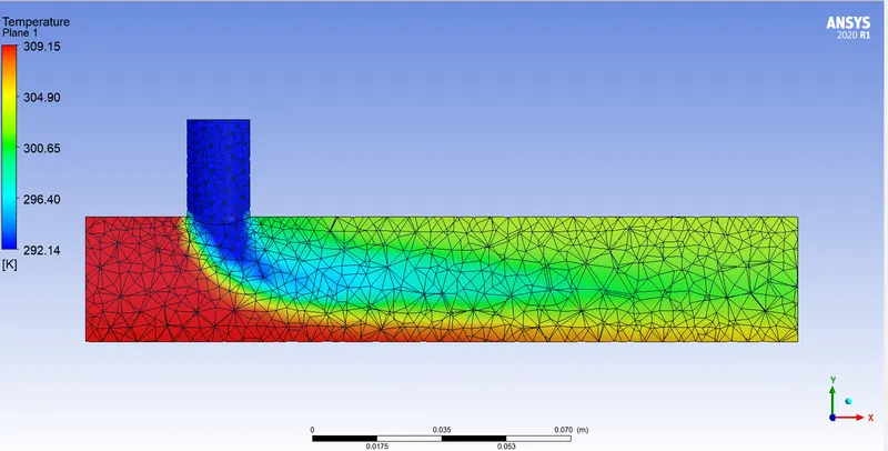
• We can clearly view from the temperature contours generated for different mesh lengths that as the mesh length is decreased the contours are getting are sharper.
• The simulation results do not change by a large margin however the results get refined.
• With the decrease in mesh length we can say that the time taken to perform simulation also increases.

Conclusion of the experiment: -

1. Effect of momentum ratio:
   • The momentum ratio played a crucial role in the mixing efficiency of the mixing tee.
   • As the momentum ratio was being increased i.e., the velocity of fluid entering from inlet-y was increased the average temperature at the outlet is reduced which indicates that the fluid have mixed more efficiently before reaching the outlet.
   • In both the cases with higher fluid velocity at inlet - y we observe lower temperature i.e., 30.250 ⁰C at outlet when momentum ratio was 2 and 27.250 ⁰C when momentum ratio was 4.
2. Effect of length
   • When the length was increased the mixture did show efficient mixing if you compare the same momentum ratio cases between shorter and longer length tee. However, in both the cases it was the increased momentum ratio that was the primary reason for efficient mixing.
   • With this, we can say that however a longer tee has more length for mixing the fluids, it is not a crucial factor for deciding the efficiency of mixing.

• In this experiment, we studied how the efficiency of a mixing tee depends upon the fluid velocity and length. With the help of ANSYS fluent, we simulated the results and found out the best conditions which can provide us with the best results.