Week 3 - External flow simulation over an Ahmed body.

AIM: To study the external flow over an ahmed body.

INTRODUCTION:

• What is an Ahmed body?

It is a 3D model that is a representative of a normal passenger car which was created to validate CFD code. We can use Ahmed body to find out different modelling stratergies because many engineers have performed a lot of experiments on it which makes it a source of rich data.

SOLVING AND MODELLING APPROACH:

• The Ahmed body will be first split as per the suggestion given using the split tool. This will improve the speed of calculations as now only half of the geometry needs to be analysed. The results would not change as the geometry is symmetric.
• We will create an enclosure for the geometry to perform external flow simulations. We will first perform a grid independence test with a coarse mesh and analyse the results that are generated. With the results that we get, we will create another enclosure to carfully capture the wake region and refine the mesh and understand the results even better.
• We will perform steady state analysis with a pressure based solver.
• We will analyse the results using CFD-post and create plots for drag coefficient to calculate the drag coefficient over the ahmed body. Using velocity and pressure contours, we will analyse the wake region.

GEOMETRY:

• We will use the import the geometry into SPACECLAIM.

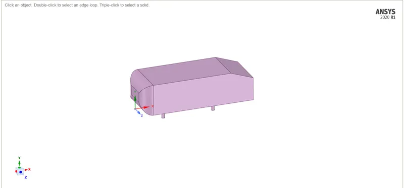
• We will create an enclosure using the enclosure feature.

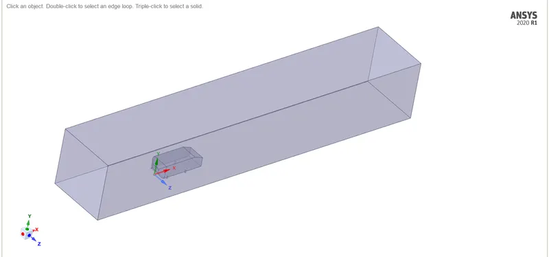
• Suppress the solid body representing the Ahmed body for all physics because we dont want to use it for meshing.
• With this you can exit the spaceclaim and perform meshing.

GRID INDEPENDENCE TEST:

At first we will use the default mesh conditions and check whether the boundary conditions gives us the accurate result after which we will refine our mesh to find out the best mesh length.

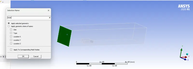
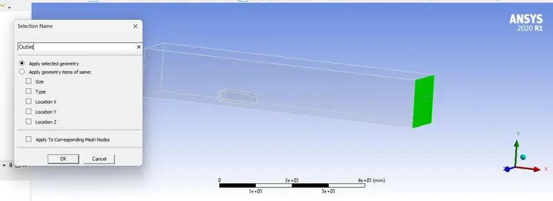
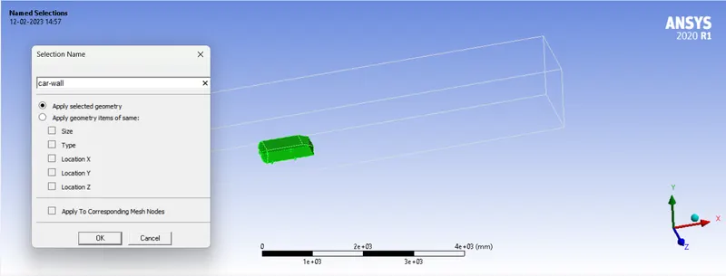
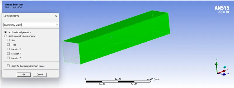
• As the geometry gets loaded, we will provide the name to the selections and hide the faces.
  • Inlet
    • 
  • Outlet
    • 
  • Car-wall
    • 
  • Symmetry-wall
    • 
• With this we can create a coarse mesh to analyse the results.

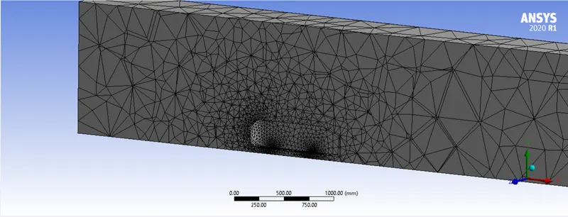
• The mesh created is good enough for the base analysis. With this, we can move to the fluent section and perform the analysis.

ANALYSIS:

• We will use pressure based solverand perform steady state analysis.

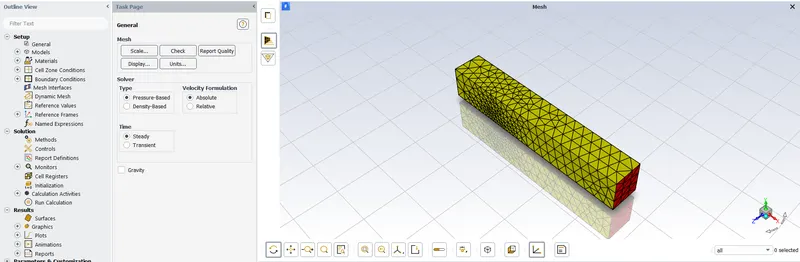
• Taking reference from the research paper given we will be using a reynolds stress model with non equillibrium wall function method for near wall treatment.
• The material to be used is Air.
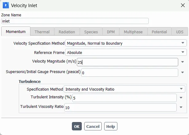
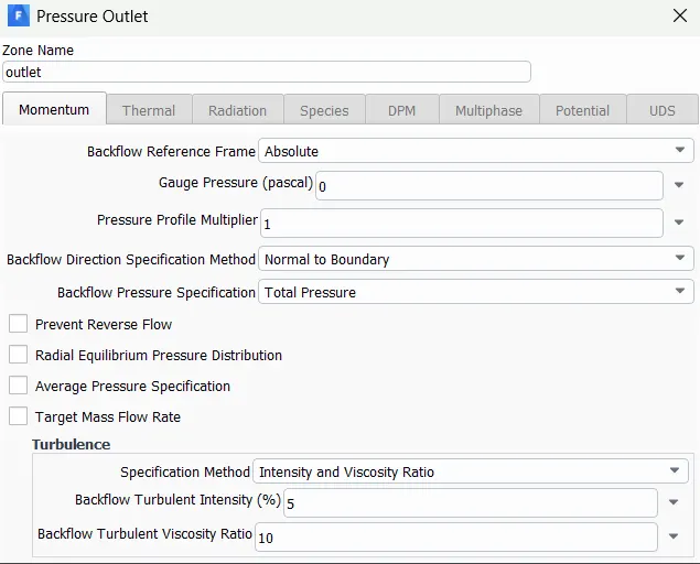
• We will provide a velocity of 25m/s at the inlet and a pressure outlet of zero gauge pressure at the outlet.
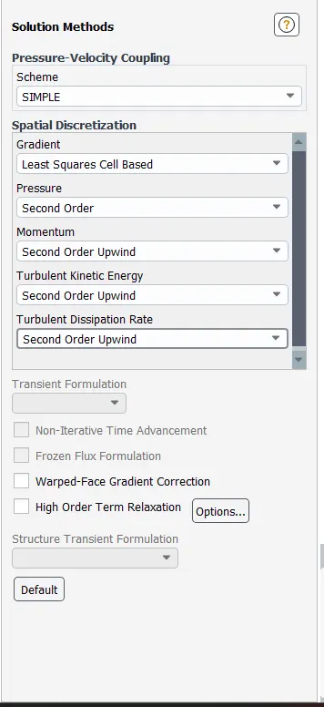
• We will be using SIMPLE scheme, second order pressure and second order upwind condition for all other variables.
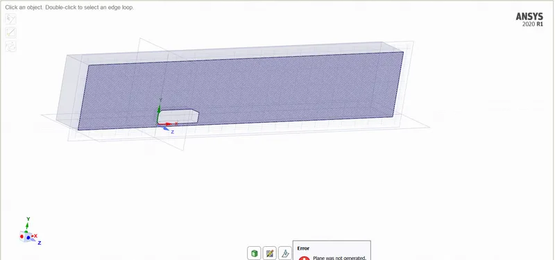
• To view the pressure and velocity contour, we will create a plane in the XY plane which is 0m away from the Z-axis.

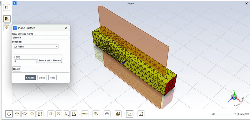
• We will create pressure and velocity contours on this z-plane. We will also create the velocity animations for both pressure and velocity.
• With all this complete, we will perform 500 iterations.

RESULTS:

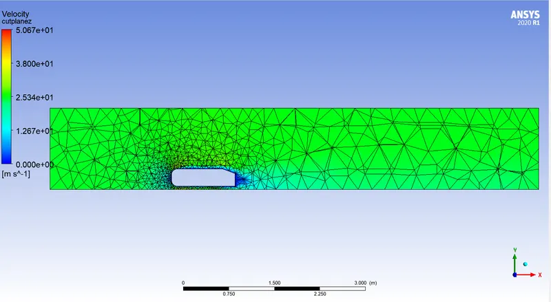
• Velocity contour:

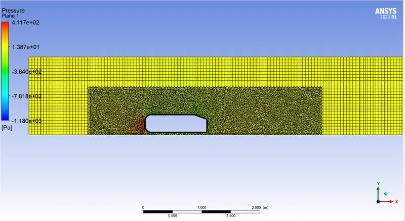
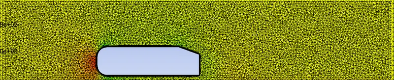
• Pressure contour:

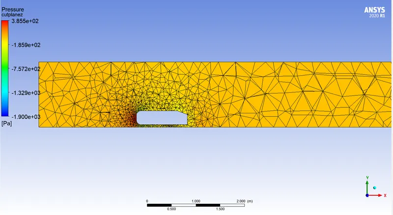
• The boundary conditions seem to provide results. Now we will improve our results by improvising the mesh around the Ahmed body and refining the mesh.

IMPROVING ENCLOSURE:

• We can see from the velocity plot that the wake region formed can be sharpenned. To do that we will create one more enclosure that will be meshed with finer elements. This way we will produce an enclosure that will generate sharp data that can be clearly visualised.
• We will open the geometry in spaceclaim and provide the enclosure as given below.

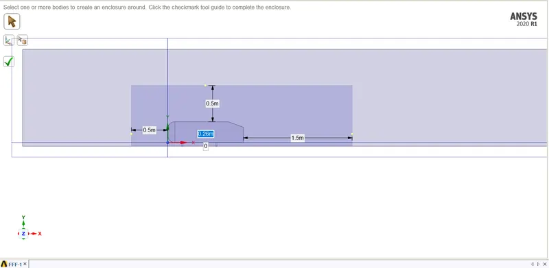
• When we look at the enclosure using section mode, we realise that the second enclosure is interferring with the first enclosure.

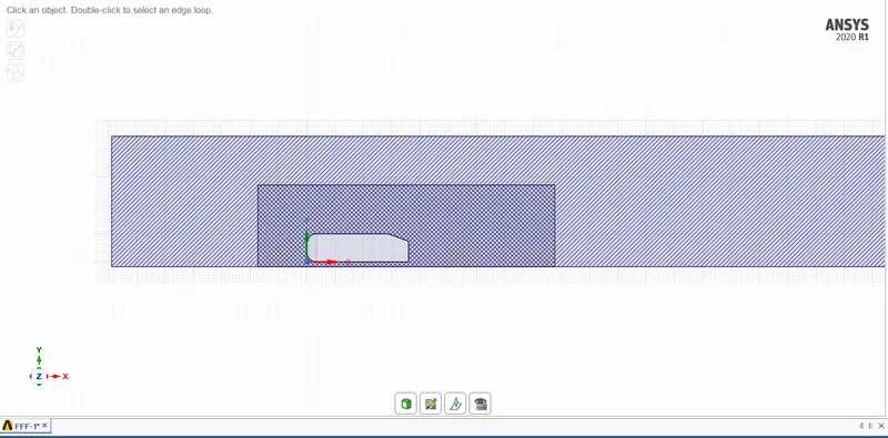
• This can create problems while meshing as the body will not be considered seperate. In order to solve this, we can use the interference feature to remove the interference between the objects.

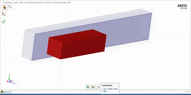
• When the interference gets solved, you can see the cross lines passing the geometry changed.

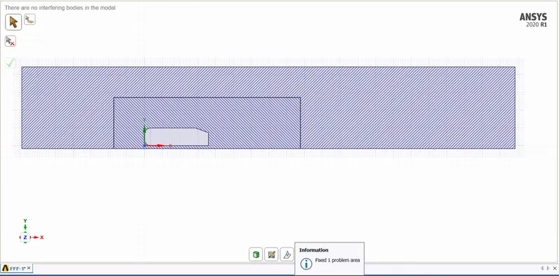
NOTE: While we did simulation for the base mesh, we forgot to make sure the share topology has been set to "share".

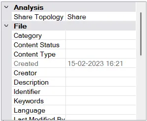
This is important to make sure the values will be shared between the enclosures.

MESHING:

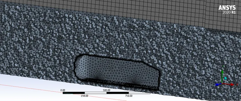
We will perform the mesh independent test for three mesh length, coarse, medium and fine and we will evaulate the effects of mesh length and find the optimal mesh length.

CASE 1:

Outer enclosure element size	100 mm
Inner enclosure element size	50 mm
Face sizing	5 mm
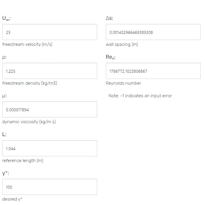
Y+	100
Number of layers	10
First layer thickness	1.4329 mm

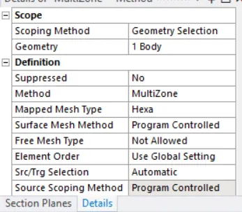
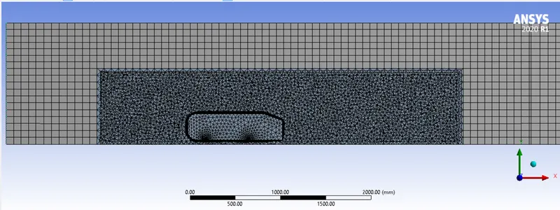
• To improve our mesh we will select the method as MULTIZONE. It will create hexahedral mesh on the areas where the mesh is possible and create tetrahedral mesh in other location.

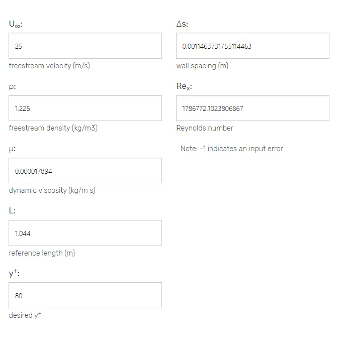
• We will use the Y+ calculator available online to calculate the first layer thickness.

• We will give 300mm mesh size to outer enclosure and the inner enclosure will be set to 60mm mesh length.

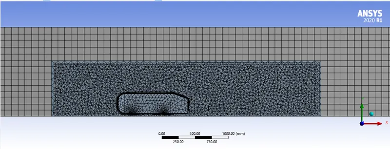
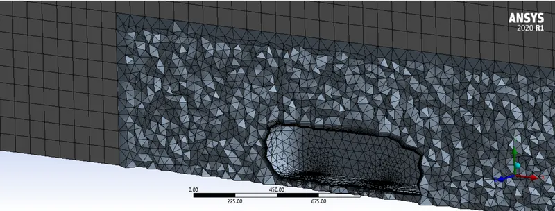
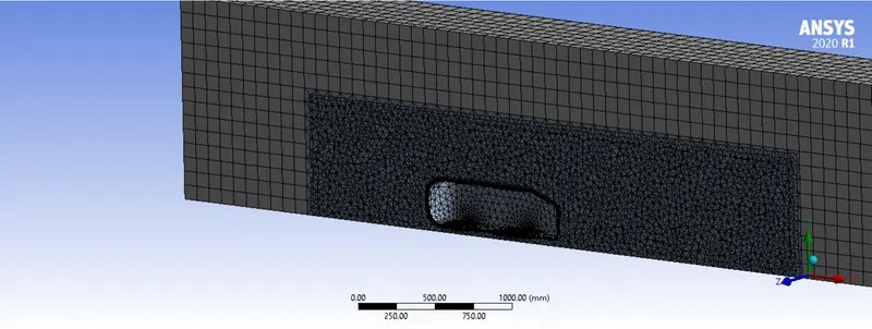
• After the mesh has been completed we will go to the fluent and give the required boundary conditions.

FLUENT DATA:

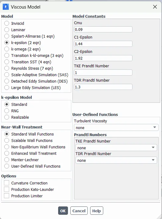
• Viscous model - K-epsilon

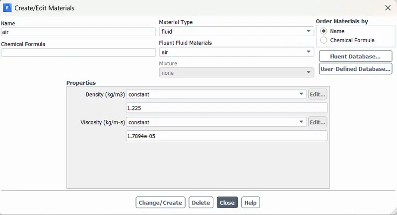
• Material - Air

• Boundary conditions:

• Referenced values:

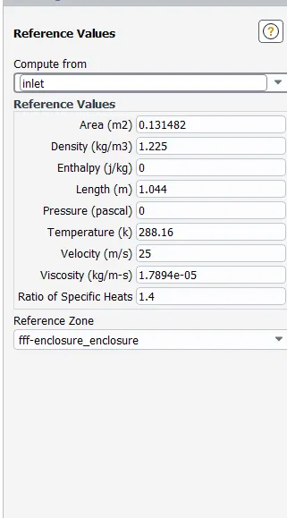
The referenced value for length is given by measuring the overall length of the ahmed body i.e., 1.044m whereas the area can be calculated by using the "Projected areas" feature of FLUENT.

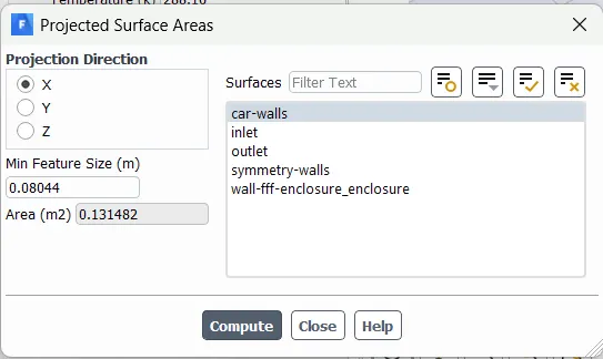
We chose the ahmed body's length and area because the result i.e., the drag coefficient needs the be calculated at the ahmed body.

• Solution method:

RESULTS:

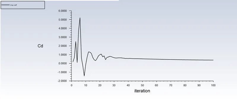
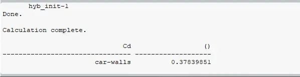
• Coefficient of drag (Cd):

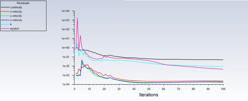
• Scaled residuals:

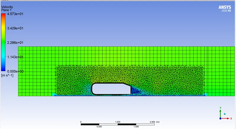
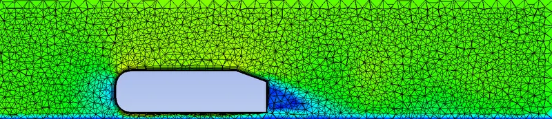
• Velocity contour:

• Pressure contour:

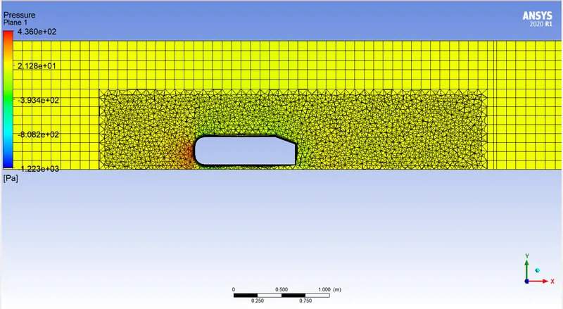
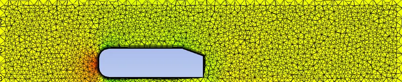
CASE - 2: MEDIUM MESH

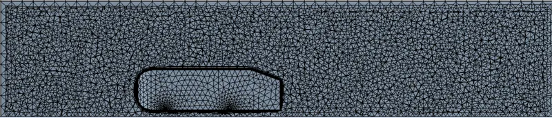
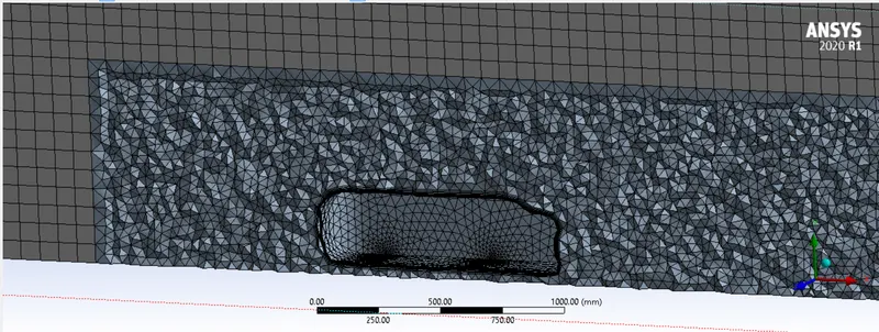
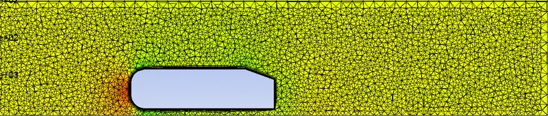
Outer enclosure element size	80 mm
Inner enclosure element size	40 mm
Face sizing	5 mm
Number of layers	10
Y+	80
First layer thickness	1.14

• We will use the same conditions in the fluent. We will run 500 iterations and run the calculation.

RESULTS:

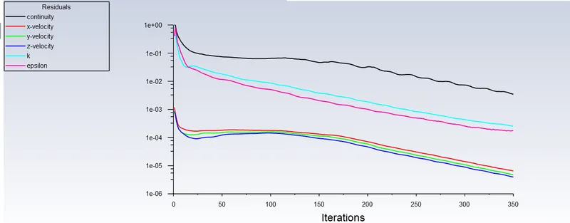
• Residual plot:

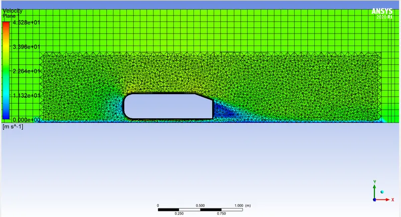
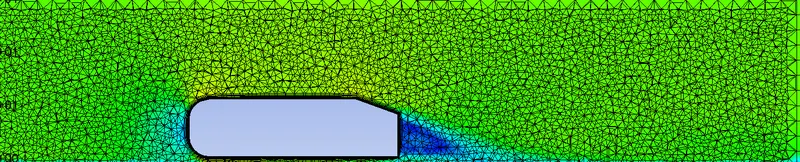
• Velocity contour:

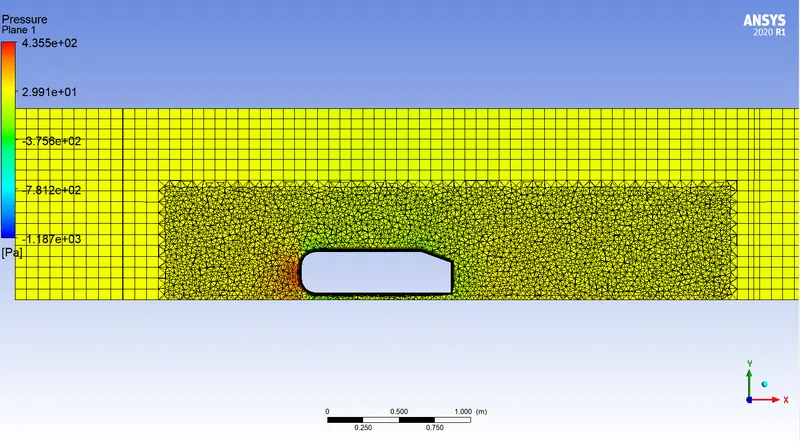
• Pressure contour:

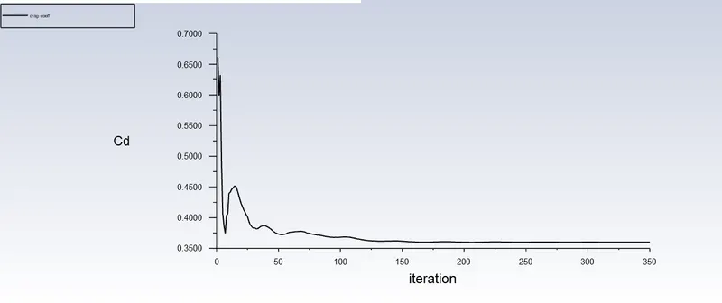
• Drag plot:

CASE - III: FINE MESH

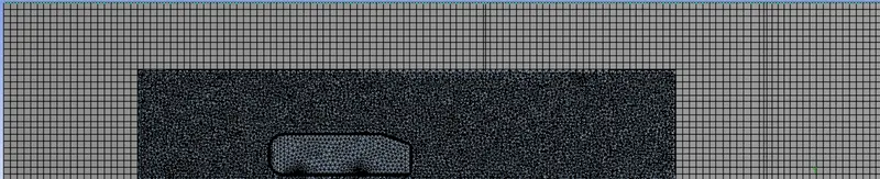
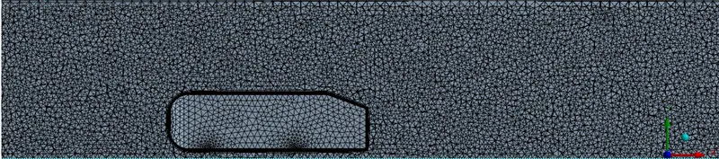
Outer enclosure element size	50 mm
Inner enclosure element size	30 mm
Face sizing	5 mm
Number of layers	10
First element size	0.859 mm
Y+	60

RESULTS:

ANALYSIS:

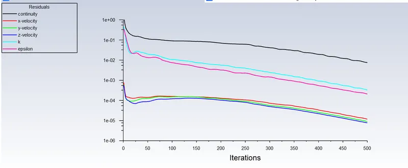
• Residuals:

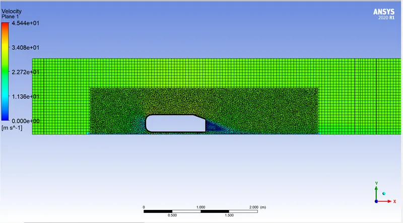
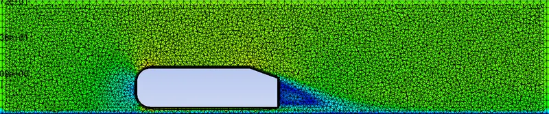
• Velocity contour:

• Pressure contour:

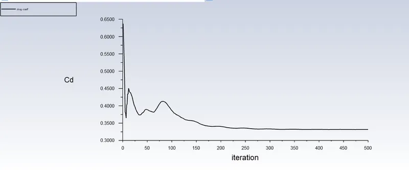
• Coefficient of drag:

CONCLUSION:

CASES	Y+	Coefficient of drag (Cd)	Number of elements
CASE - I : Medium mesh	100	0.37	2,58,511
CASE - II : Fine mesh	80	0.36	4,52,334
CASE - III : Ultra fine mesh	60	0.33	10,76,410

OVERALL RESULT:

• With the experiment we realised the reason why negetive pressure is formed in the wake region. When the vehicle movies through a fluid, the fluid resists the movement by imparting viscous forces onto the vehicle. When the fluid reaches the rear end of the vehicle due to the sudden change in geometry the flow gets seperated. This seperation of flow causes a negetive wake to be formed behind the vehicle.
• This negetive wake creates a suction force at the rear end of the vehicle which adds up to the drag force produced at the front of the vehicle increasing the overall drag that the vehicle experiences.
• The point of seperation is formed at the rear of the ahmed body. Point of seperation is the area where the boundary layer lifts off from the surface. The point of seperation is mainly caused due to sudden changes in geometry which in turns results in the formation of a negetive pressure wake.
• The drag coefficient is dependent upon the number of elements and Y+ value created at the ahmed body. As the Y+ value was getting reduced, the first element distance from the walls were changing which implies that to get accurate results. We need to have the exact Y+ value.