Week 2 - Flow over a Cylinder.

AIM: To study the flow over a cylinder and understand karmen vortex street.

THEORY:

What is a vortex?

A vortex is a mass of fluid moving in a circular motion that tends to form a cavity or vaccum at the centre. Whenever a body is nearby a vortex, the general behaviour is to be attracted to the vaccum present at the centre.

The general example of formation of vortex in nature will be tornadoes, whirlpool etc.

What do you mean by karmen vortex street?

Whenever a fluid flows over a blunt surface at a particular flow velocity and within a range reynold number, there is a repeating pattern of vorticies that are being formed behind the surface due to vortex shedding. This pattern is called as karmen vortex street. It is responsible for unsteady seperation of flow of fluid around a blunt surface.

What is vortex shedding?

Vortex shedding as you can observe in the image given below is an oscillating moment of fluid that takes place when the fluid flows over a blunt surface such as a cylinder at certain velocities. Vortex shedding is dependent upon the reynolds number.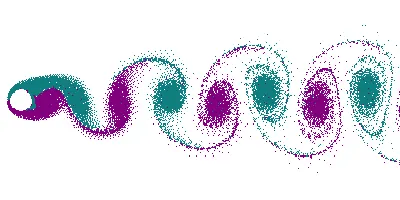

What is Strouhal number?

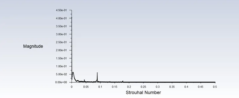
The strouhal number is a dimensionless number used for analyzing unsteady fluid flow dynamic problems.

The strouhal number can be represented as,

• St = f*L / v where,
• f: frequency
• L: Length
• V: Flow velocity

SOLVING AND MODELLING APPROACH:

The main objective of the study is to understand the flow over a blunt surface (a cylinder) at different reynold number and capture the various information related to the flow parameters like vortex shedding, coefficient of drag & lift, calculating strouhal number etc.

In order to gather information related to the above mentioned parameters our simulation will be bi-furcated into two parts both in which we will perform steady and unsteady state simulations. In the first part, we will simulate the flow through a cylinder for a reynold's number of 100 and calculate the strouhal number. In the second part, we will simulate the flow for a variety of reynold number that ranges from 10 to 1,00,000. We will evaluate the lift and drag coefficients as well.

First we will create the 2D geometry of the model using spaceclaim and mesh the geometry in the meshing module. We will keep the mesh to be fine in order to capture finite details of the results. We will provide inflation layer to the cylinder as that is the region where we want to observe the vortex shedding.

For the boundary conditions, the material to be used will be user specified with a specific density and viscocity which will be kept constant through out the simulation. With constant fluid parameter, constant diameter and varying Reynolds number, we will be able to calculate the varying velocity.

The calculated velocity will be used at the inlet (Velocity inlet). Outlet will be given a pressure outlet i.e., gauge pressure. The walls i.e., the cylinder surface will be given no-slip condition.

PROCEDURE:

Geometry:

• We will open ANSYS Workbench and open Spaceclaim to create our geometry.

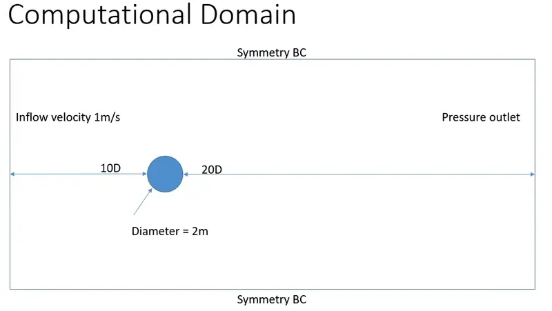
Note:- The image has been taken from internet

• Now, we will create sketch for the geometry in Spaceclaim.

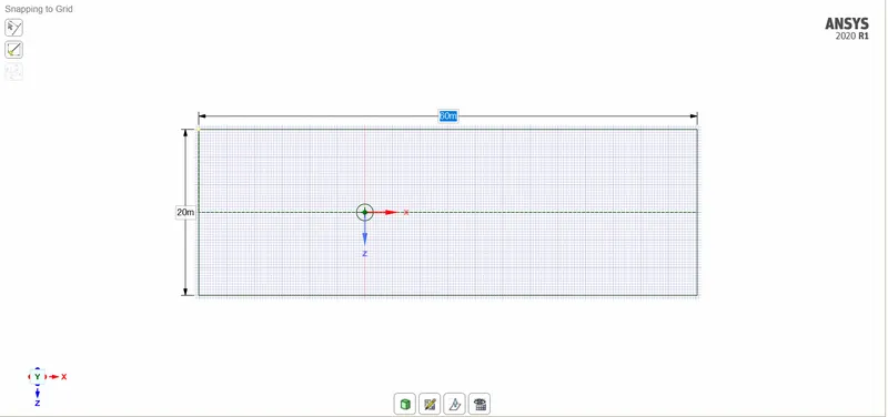
• As the sketch has been made, we can use the pull feature to create a surface.
• After we create the surface, we will delete the inner circle and create a hole there and also delete all the construction lines.

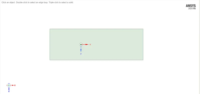
• Once the geometry has been created, we will mesh the created surfaces for flow simulations. We will open the meshing window and update the geometry.

MESHING:

• Once we update the surface inside meshing, we will observe a default quadrilateral mesh being formed. Since we need to measure results very precisely we will change the mesh type to triangles.

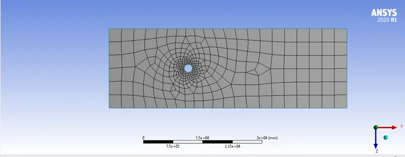
• To perform this function, we will use the method feature and select triangles instead of quadrilateral.

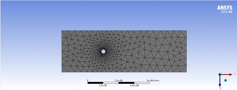
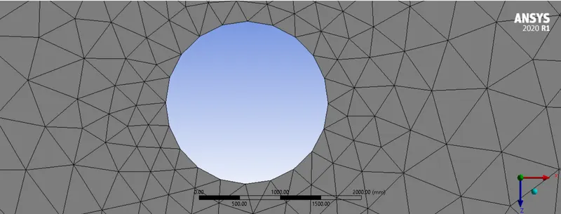
• When we zoom to the cylinder section, we observe the circular cross section of the circle to be formed as a polygon with multiple sides. We cannot have this because we need to perform flow analysis of the circular region and the polygonal sides will cause flow seperation to take place.

• To smoothen the cylinder surface, we will use the sizing feature and increase the number of divisions of the boundary of the cylinder which will give us a more refined geometry.

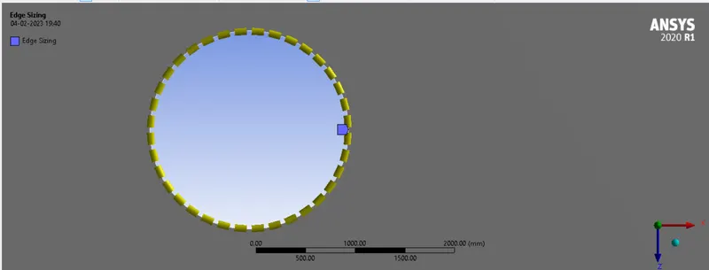
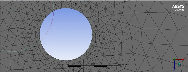
• Now the surface that has to be studied has been refined. We can improve the results around the area by using a inflation layer which will refine the mesh quality in the cylinder surface.

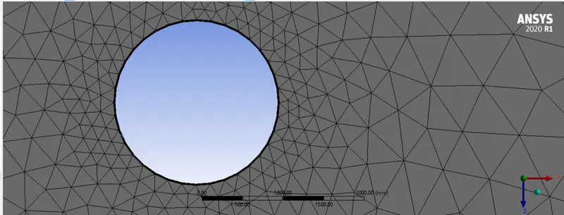
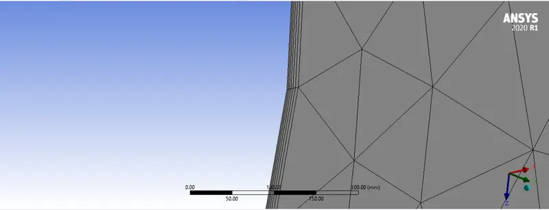
• We can see how refined the surface looks after providing the inflation.
• We will now provide a mesh length of 0.5m and generate the mesh.

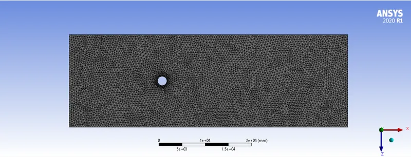
• With the mesh done, the final task is to provide the boundary conditions.

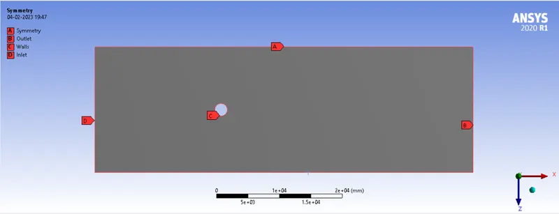
• After that we can move to the fluent module to provide the boundary conditions for different cases.

CASE - I: Simulate steady and unsteady flow with Re = 100 and calculate strouhal number.

Before moving forward with the boundary conditions, we need to calculate the inlet velocity. We have been given the value of Reynold's number for our case.

`R e = (ρ V L)/μ`

Where:

Re = Reynold's number = 100

ρ = Density = 1 kg/m3

v = Velocity

L = Charecteristic length = D = 2m.

μ = Viscosity = 0.02

With the following values, we can calculate the value of velocity at inlet

Inlet velocity (v) = 1m/s.

• We can now move to the Fluent section and input the necessary models and boundary conditions for our analysis.

SIMULATION:

Steady state

• After we open fluent, we first check the mesh using the check mesh feature.
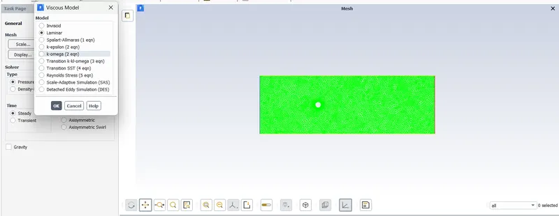
• After the mesh check, we can move to the PHYSICS tab to select our model. We will be using a steady state analysis with a laminar model.

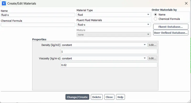
• After the model, we will create a new material with the density and viscosity according to our case.
• We will make sure that we delete all other material and only set the newly created material at the cell zone condition.

• After this, we will set our boundary conditions.
  
  1. Inlet (velocity inlet): 1m/s
  2. Outlet (pressure outlet): 0 gauge pressure
  3. Walls: No slip condition.
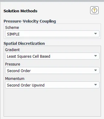
• With the boundary condition set, we need to select the following solution method

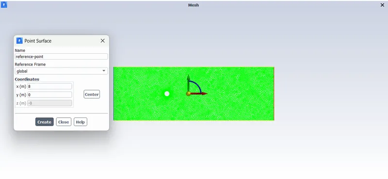
• We will create a point at 4 times the diameter of the cylinder at the right side of the surface. This point will be used as the reference point for measuring/observing the velocity.

• We will create three plots while the simulation is being performed
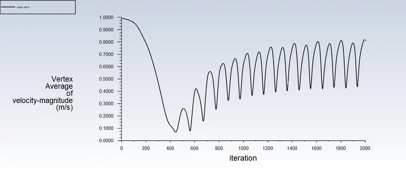
  1. Vertex average for velocity magnitude
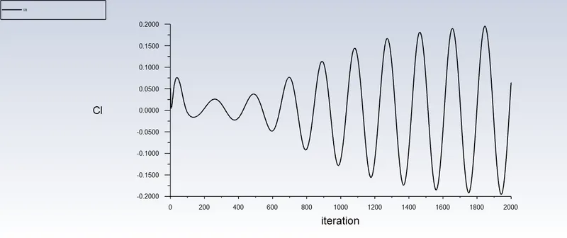
  2. Lift coefficient around the cylinder/wall.
  3. Drag coefficient around the cylinder/wall.
• We will create vertex average of velocity at the reference point.
• We will create the drag and lift coefficient at walls.
• Before initialising the solution, we will uncheck the convergence criteria.

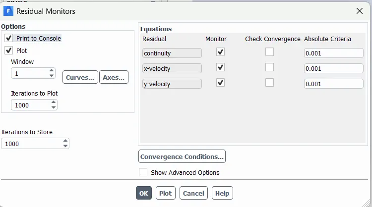
• With this, we will perform 1000 iterations at first and calculate the velocity plots.

RESULTS:

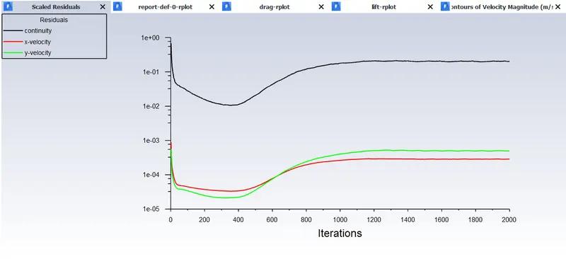
Scaled residuals

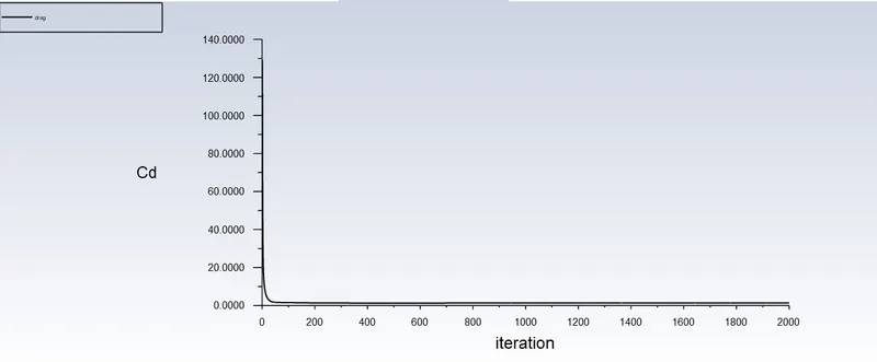
Drag coefficient at walls

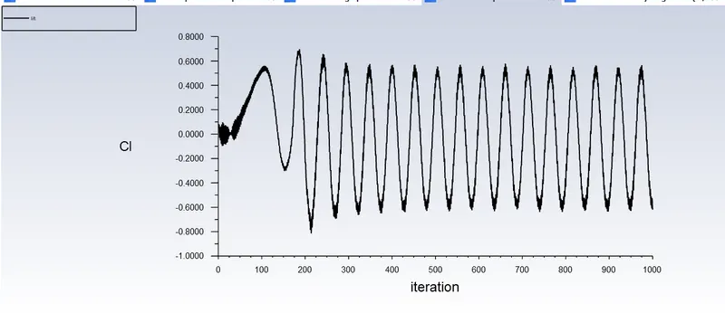
Lift coefficient at walls

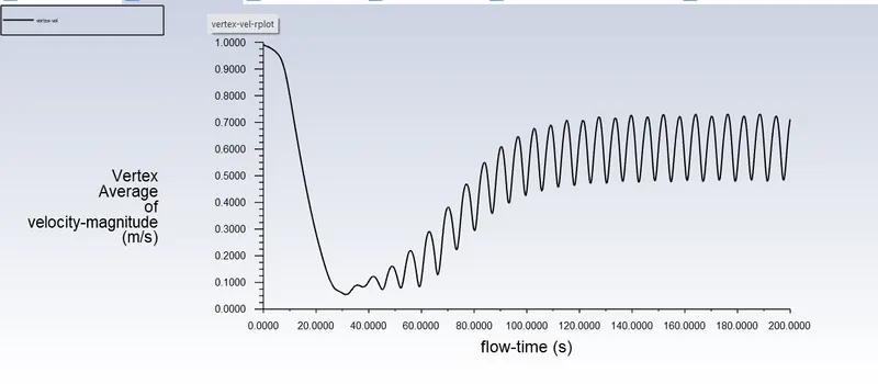
Vertex average of velocity at reference point

Strouhal number:

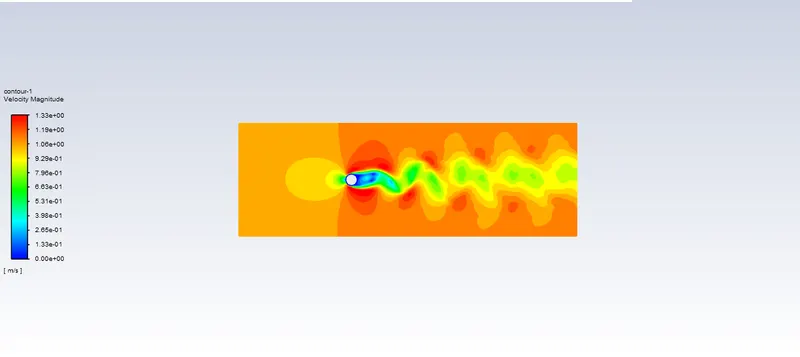
Velocity contour:

Unsteady state:

For unsteady state simulation we will replace the model to a turbulent model in the general section and with the same boundary conditions we will calculate our results.

We will generate the same plots that we generated for the steady state problems.

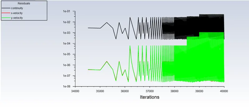
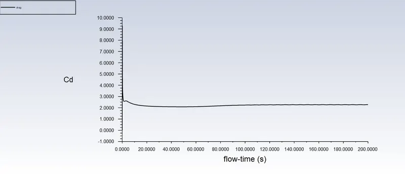
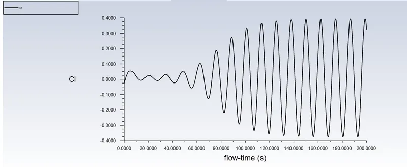
We have used a time step size of 0.1 second and the number of time steps as 1600 iterations. We had to use 1600 iterations because the solution took time to converge.

RESULTS:

Scaled residuals

Vertex average of velocity at reference point

Drag coefficient at walls

Lift coefficient at walls

Strouhal number

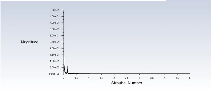
Velocity contour

CASE - II: Calculate the coefficient of drag and lift over a cylinder by setting the Reynolds number to 10,100,1000,10000 & 100000.

• We will use the same geometry that was used for case - 1. We will do this by sharing the geometry as shown below.

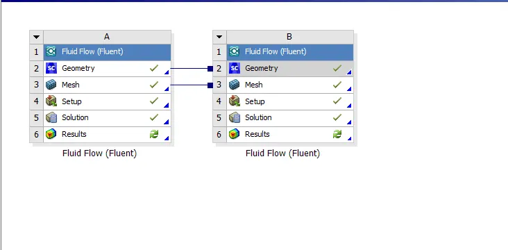
• In this case, we need to perform the simulation for different values of Re.
• The fluid properties will remain same, the only thong changing will be velocity.
• The velocity for different reynolds number are given below:
  • Re = 10, v = 0.1 m/s
  • Re = 100, v = 1 m/s
  • Re = 1000, v = 10m/s.
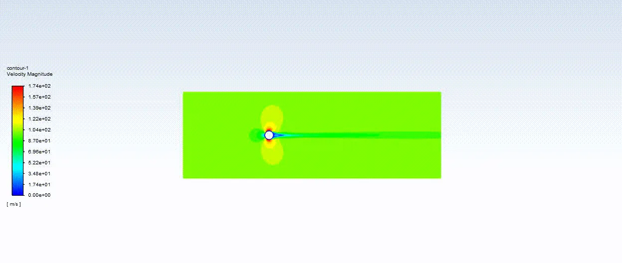
  • Re = 10,000, v = 100 m/s.
  • Re = 1,00,000, v = 1000 m/s.

RESULTS:

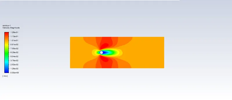
Velocity contour:

• Re = 10

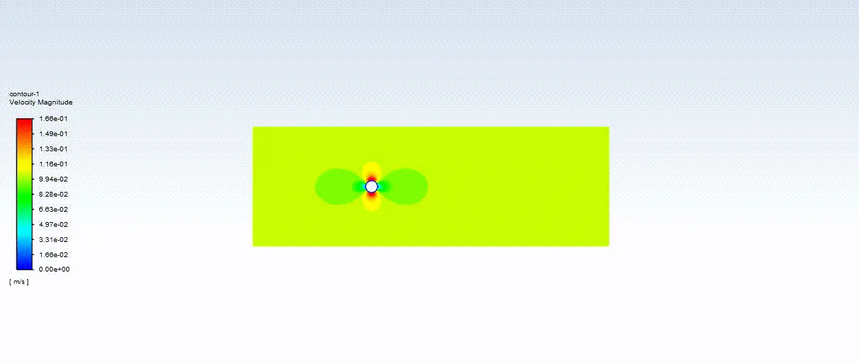
• Re = 100

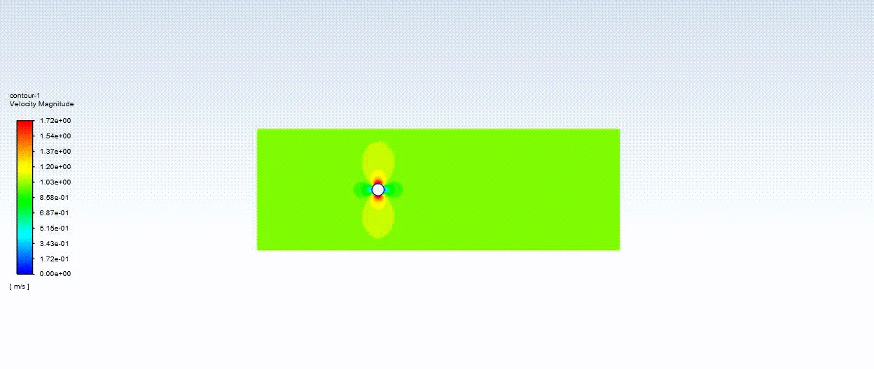
• Re = 1000

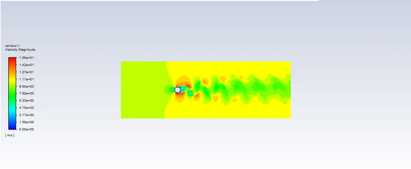
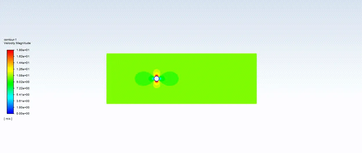
• Re = 10000

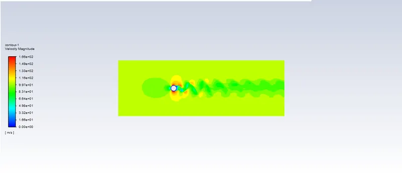
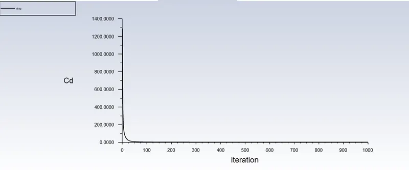
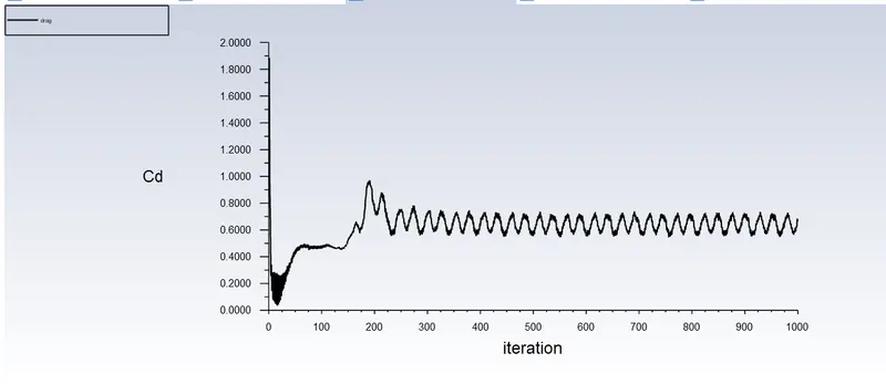
Drag coefficient

• Re = 10

• Re = 100

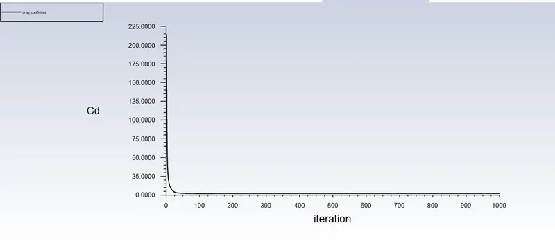
• Re = 1000

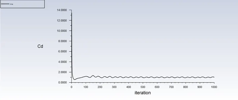
• Re = 10000

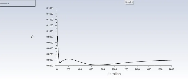
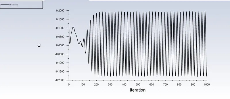
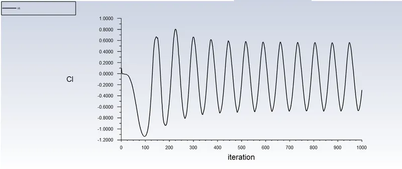
Lift coefficient

• Re = 10

• Re = 100

• Re = 1000

• Re = 10000

CONCLUSION:

1. As the reynold number is increasing, the wake formed behind the cylinder gets bigger and bigger.
2. From the images, it is clearly visible that as the reynold number is increasing the coefficient of lift and drag also increases.