Week 5.1 - Mid term project - Solving the steady and unsteady 2D heat conduction problem
AIM: Solving steady state and unsteady state 2D heat convection equation
The 2D heat conduction equation is given by:
`(delT)/(delt) = alpha*((del^2T)/(delx^2) + (del^2T)/(dely^2))`
Boundary conditions:
The following information has been given about the domain:
- Top Boundary = 600 K
- Bottom Boundary = 900 K
- Left Boundary = 400 K
- Right Boundary = 800 K
We will perform the steady state and transient analysis for the convection equation.
THEORY:
1. STEADY STATE ANALYSIS:
Steady state analysis means solving the convective portion of the convection equation i.e., the terms independent of t.
`(del^2T)/(delx^2) + (del^2T)/(dely^2) = 0`
In order to solve this equation using matlab, we will convert the equation into algebric form.
Therefore, the following equation can be written as
`(T_l -2* T_p +T_r)/(dx^2) + (T_t - 2*T_p + T_b)/dy^2 = 0`
where,
`T_l = T(i-1,j)`
`T_p = T(i,j)`
`T_r = T(i+1,j)`
`T_b = T(i,j-1)`
`T_t = T(i,j+1)`
2. TRANSIENT STATE ANALYSIS:
When we solve the time dependent terms, it's called transient state analysis.
The equations can be solved by using Jacobian method, Gauss seidal method, and SOR method.
Jacobian method:
Jacobian method is an iterative method used to solve linear equations. In this, we take an initial assumption of the value being calculated and then solve the equation untill the solution converges.
Gauss-seidel method:
The difference between the Gauss–Seidel and Jacobi methods is that the Jacobi method uses the values obtained from the previous step while the Gauss–Seidel method always applies the latest updated values during the iterative procedure.
SOR method:
This iterative method uses a value `omega`(omega) to guess the value for next iteration. By employing the below mentioned formula the values are computed.
`T(i,j) = (1-omega)*Told(i,j) + (omega)*(T_(GS))`
We can also use jacobian method instead of gauss seidel method.
Explicit vs Implicit solvers:
1. Explicit solvers:
When the equation being studied is calculated for previous time step it's called explicit solution i.e., n.
2. Implicit solvers:
When the equation being studied is calculated for next time step it's called as implicit solution i.e., n+1.
SOLVING:
1. Solving steady state equation:
For steady state portion, we will be solving
`(del^2T)/(delx^2) + (del^2T)/(dely^2) = 0`
This equation can be written as
`(T_l -2* T_p +T_r)/(dx^2) + (T_t - 2*T_p + T_b)/dy^2 = 0`
When we re-arrange the Tp term to the left and other terms to the right, we get the following equation
`T_p = 1/K*(T_l + T_r)/(dx^2) + 1/K*(T_b + T_t)/(dy^2)`
where
`K = 2*((dx^2 + dy^2)/(dx^2*dy^2))`
- This equation has to be solved using Jacobian, Gauss seidel and SOR method. I have included all the methods of solving in a single code.
CODE:
close all
clear all
clc

%number of nodes in x and y
nx = 10;
ny = 10;

%dimensions of the domain
x = linspace(0,1,nx);
dx = x(2) - x(1);
y = linspace(0,1,nx);
dy = x(2) - x(1);

%constants:
k = 2*((dx^2 + dy^2))/((dx^2)*(dy^2));
tol = 1e-4;
error = 9e9;
iterative_solver = 3;
jacobian_iter = 1;
GS_iter = 1;
SOR_iter = 1;
omega = 1.5;

%Temperature within domain
T = 300*ones(nx,ny);
T(1:end, 1) = 400;
T(1:end, end) = 800;
T(1,1:end) = 600;
T(end, 1:end) = 900;

%Temperatures' at the corner points
T(1,1) = 500;
T(1,end) = 700;
T(end,end) = 850;
T(end, 1) = 650;

Told = T;

%JACOBIAN METHOD
if(iterative_solver == 1)
    while (error > tol)
        for i = 2 : nx-1
            for j = 2 : ny-1
                term_1 = (Told(i-1,j) + Told(i+1, j))/(k*dx^2);
                term_2 = (Told(i,j-1) + Told(i,j+1))/(k*dy^2);
                T(i,j) = term_1 + term_2;
            end
        end
        error = max(max(abs(Told - T)));
        Told = T;
        jacobian_iter = jacobian_iter + 1;

        %GRAPH
        figure(1)
        colormap(jet);
        A = contourf(x,y,T);
        clabel(A);
        set(gca, 'Ydir', 'reverse');
        xlabel('x - axis');
        ylabel('y - axis');
        title_text = sprintf('Iteration number = %d', jacobian_iter);
        title(title_text);
    end
end

%GAUSS - SEIDEL METHOD
if (iterative_solver == 2)
    while (error > tol)
        for i = 2:nx-1
            for j = 2:ny-1
                term_1 = (T(i-1,j) + Told(i+1,j))/(k*dx^2);
                term_2 = (T(i,j-1) + Told(i,j+1))/(k*dy^2);
                T(i,j) = term_1 + term_2;
            end
        end
        error = max(max(abs(Told - T)));
        Told = T;
        GS_iter = GS_iter + 1;

        %GRAPH
        figure(2)
        colormap(jet);
        B = contourf(x,y,T);
        clabel(B);
        xlabel('X-axis');
        ylabel('Y-axis');
        set(gca, 'Ydir', 'reverse');
        title_text = sprintf('Iteration number = %d', GS_iter);
        title(title_text);
    end
end

%SOR METHOD
if(iterative_solver == 3)
    while(error > tol)
        for i = 2:nx-1
            for j = 2:ny-1
                term_1 = (T(i-1,j) + Told(i+1,j))/(k*dx^2);
                term_2 = (T(i,j-1) + Told(i,j+1))/(k*dy^2);
                T(i,j) = ((1-omega)*(Told(i,j))) + ((omega)*(term_1+term_2));
            end
        end
        error = max(max(abs(Told - T)));
        Told = T;
        SOR_iter = SOR_iter + 1;

        %GRAPH
        figure(3)
        colormap(jet);
        C = contourf(x,y,T);
        clabel(C);
        set(gca, 'Ydir', 'reverse');
        xlabel('x-axis');
        ylabel('y-axis');
        title_text = sprintf('Iteration number = %d', SOR_iter);
        title(title_text);
    end
end
Explaination of the code:
- The domain is a 1m x 1m square domain where the the temperature conditions at the four boundaries are same as the one given in question.
- In the jacobian method, the old values of temperature are used to calculate the next values as at the instant of solving, we dont have information of the next point.
- In the gauss seidel method, values for next point are taken as soon as they are available to us.
- In the SOR method, we use a function called omega, which is used to calculate the next value. We have used gauss seidel to assist SOR method.
- The methods are inside a if loop, which can be used by changing the value of the variable used for the if loop which is 'iterative_solver'.
- We can use jacobian, gauss seidel and SOR method with iterative_solver as 1,2 and 3 respectively.
RESULTS:
1. Jacobian method:
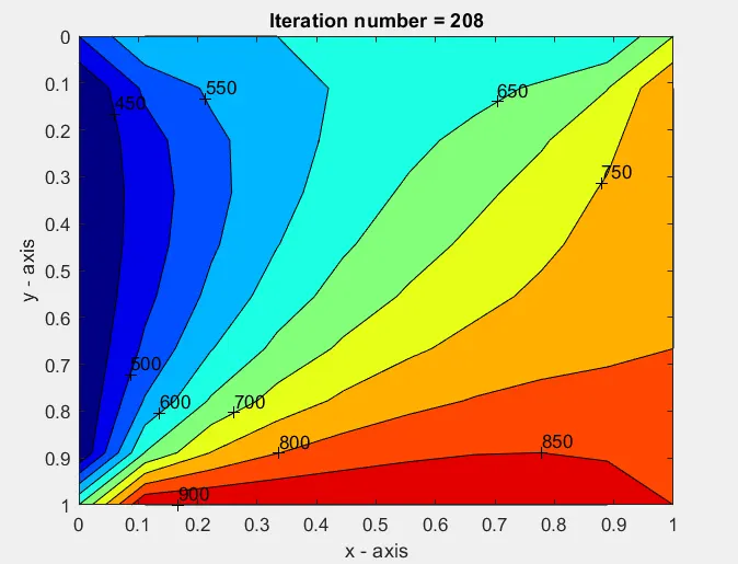
- Number of iteration = 208
2. Gauss seidel method:
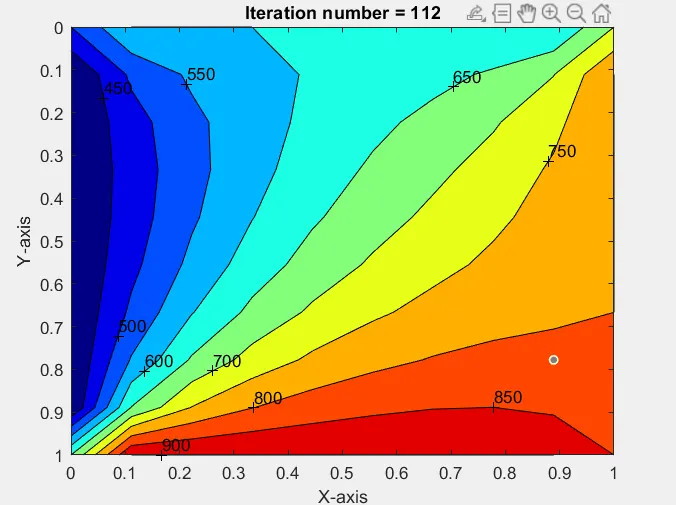
- Number of iterations = 112
3. SOR method:
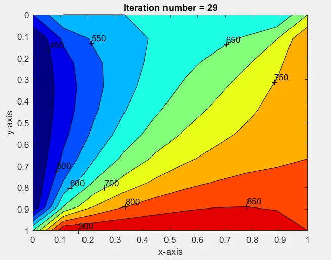
- Number of iterations: 29
2. Transient state analysis:
In the analysis, we will include the time term during calculation.
We know,
`(delT)/(delt) = alpha*((del^2T)/(delx^2) + (del^2T)/(dely^2))`
If we convert the above equation into algebric form, we get
`(T_p^(n+1) + T_p^(n))/(dt) = (alpha)*((T_l - 2*T_b + T_r)/(dx^2) + (T_b - 2*T_p + T_t)/dy^2)^(n)`
- When we are taking the power as 'n', the method is called explicit and when we take 'n+1' it is implicit.
1. Explicit method:
`(T_p^(n+1) + T_p^(n))/(dt) = (alpha)*((T_l - 2*T_b + T_r)/(dx^2) + (T_b - 2*T_p + T_t)/dy^2)^(n)`
The equation can be re-written as
`T_p^(n+1) = T_p^(n) + k_1(T_l - 2T_p+ T_r)^n + k_2(T_T - 2*T_p + T_b)^n`
where,
`k_1 = alpha*(dt/dx^2)`
`k_2 = alpha*(dt/(dy^2))`
Here, k1 and k2 are also called as the CFL for the equation.
For explicit diffusion problems, we need to make sure the sum of k1 and k2 i.e., CFL should be less than or equal to 0.5.
`CFL <= 0.5`
2. Implicit method:
`(T_p^(n+1) + T_p^(n))/(dt) = (alpha)*((T_l - 2*T_b + T_r)/(dx^2) + (T_b - 2*T_p + T_t)/dy^2)^(n+1)`
The equation can be re-written as
`T_p^(n+1) = 1/(1+2*k1 +2*k2) * (T_p^n + k1*(T_l + T_r)^(n+1) + k2*(T_t + T_b)^(n+1))`
Code for explicit method for transient analysis:
clear all
close all
clc

nx = 10;
ny = 10;
dt = 0.002;
nt = 500;

x = linspace(0,1,nx);
dx = x(2) - x(1);
y = linspace(0,1,ny);
dy = y(2) - y(1);

%defining temperature
T = 300*ones(nx, ny);
T(1:end, 1) = 400;
T(1:end, end) = 800;
T(1,1:end) = 600;
T(end, 1:end) = 900;

%Temperatures at the corner points
T(1,1) = 500;
T(1,end) = 700;
T(end,end) = 850;
T(end, 1) = 650;

Told = T;

%constants:
alpha = 1.4;
k1 = (alpha)*(dt/(dx^2));
k2 = (alpha)*(dt/(dy^2));
CFL = k1 + k2;


for k = 1:nt
    for i = 2 : nx - 1
        for j = 2 : ny-1
                T(i,j) = (Told(i,j)) + k1*(Told(i-1,j) - 2*Told(i,j) + Told(i+1,j)) + k2*(Told(i,j-1) - 2*Told(i,j) + Told(i,j+1));
        end
    end
        Told = T;

        figure(1)
        colormap(jet);
        A = contourf(x,y,T);
        clabel(A);
        set(gca, 'Ydir', 'reverse');
        xlabel('X-axis');
        ylabel('Y-axis');
        title_text = sprintf('Number of timesteps = %d', nt);
        title(title_text);
end
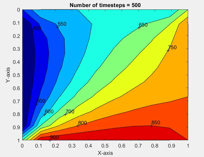
Result:
Code for implicit method for transient analysis:
clear all
close all
clc

nx = 10;
ny = 10;

x = linspace(0,1,nx);
dx = x(2) - x(1);
y = linspace(0,1,ny);
dy = y(2) - y(1);
dt = 0.001;

%constant:
alpha = 1.4;
k1 = (alpha)*(dt/(dx^2));
k2 = (alpha)*(dt/(dy^2));
CFL = k1+k2;
tol = 1e-4;
iter_no = 1;
iteration = 3;

%temperature domain
T = 300*ones(nx,ny);
T(1,1:end) = 600;
T(end, 1:end) = 900;
T(1:end, 1) = 400;
T(1:end, end) = 800;
T(1,1) = 500;
T(end,end) = 850;
T(1,end) = 700;
T(end, 1) = 650;

Told = T;
Tprev = T;


%JACOBIAN
if iteration == 1
    for k = 1:1500
        error = 9e9;
        while(error > tol)
            for i = 2:nx-1
                for j = 2:ny-1
                    term_1 = 1/(1+2*k1+2*k2);
                    term_2 = k1*term_1;
                    term_3 = k2*term_1;
                    T(i,j) = (term_1)*(Tprev(i,j)) + (term_2)*(Told(i-1,j) + Told(i+1,j)) + (term_3)*(Told(i,j-1) + Told(i,j+1));
                end
            end
            error = max(max(abs(Told-T)));
            Told = T;
            iter_no = iter_no + 1;

            %GRAPH
            figure(1)
            colormap(jet);
            A = contourf(x,y,T);
            clabel(A);
            set(gca, 'Ydir', 'reverse');
            xlabel('X-axis');
            ylabel('Y-axis');
            title_text = sprintf('Iteration number = %d', iter_no);
            title(title_text);
        end
        Tprev = T;
    end
end

%GAUSS SEIDEL
if (iteration == 2)
    for k = 1:1500
        error = 9e9;
        while(error > tol)
            for i = 2:nx-1
                for j = 2:ny-1
                    term_1 = 1/(1+2*k1+2*k2);
                    term_2 = k1*term_1;
                    term_3 = k2*term_1;
                    T(i,j) = (term_1)*(Tprev(i,j)) + (term_2)*(T(i-1,j) + Told(i+1,j)) + (term_3)*(T(i,j-1) + Told(i,j+1));
                end
            end
            error = max(max(abs(Told - T)));
            Told = T;
            iter_no = iter_no + 1;

            %GRAPH
            figure(2)
            colormap(jet);
            B = contourf(x,y,T);
            clabel(B);
            set(gca, 'Ydir', 'reverse');
            xlabel('X-axis');
            ylabel('Y-axis');
            title_text = sprintf('Iteration number = %d', iter_no);
            title(title_text);

        end
        Tprev = T;
    end
end

%SOR method
if(iteration == 3)
    omega = 1.1;
    for k = 1:1500
        error = 9e9;
        while(error > tol)
            for i = 2: nx-1
                for j = 2: ny - 1
                    term_1 = 1/(1+2*k1+2*k2);
                    term_2 = k1*term_1;
                    term_3 = k2*term_1;
                    T(i,j) = ((1-omega)*Told(i,j)) + omega*((term_1*Tprev(i,j)) + (term_2*(Told(i+1,j)+T(i-1,j))) + (term_3*(T(i,j-1)+Told(i,j+1))));
                    %T(i,j) = ((1-omega)*(Told)) + (omega)*((term_1*(Tprev(i,j)) + (term_2*(T(i-1,j) + Told(i+1,j))) + (term_3*(T(i,j-1) + Told(i,j+1)))));
                end
            end
            error = max(max(abs(Told - T)));
            Told = T;
            iter_no = iter_no + 1;

            %GRAPH
            figure(3)
            colormap(jet);
            C = contourf(x,y,T);
            clabel(C);
            set(gca, 'Ydir', 'reverse');
            xlabel('X-axis');
            ylabel('Y-axis');
            title_text = sprintf('Iteration number = %d', iter_no);
            title(title_text);
        end
        Tprev = T;
    end
end
Result for implicit method:
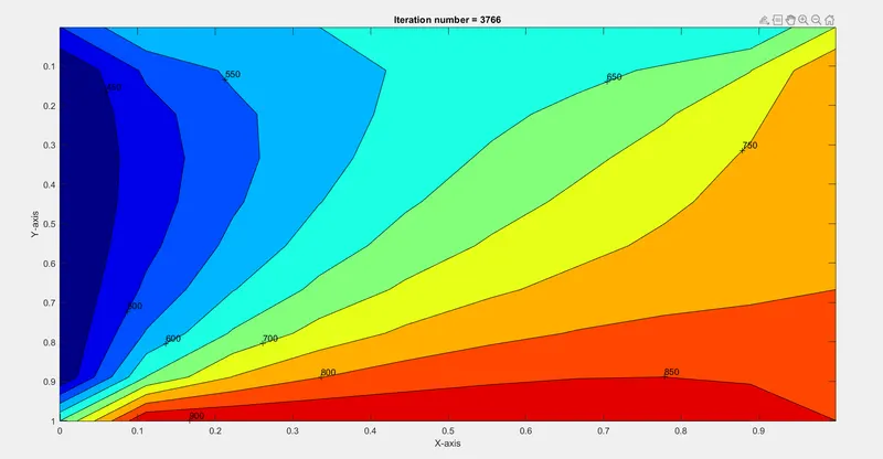
1. Jacobian method
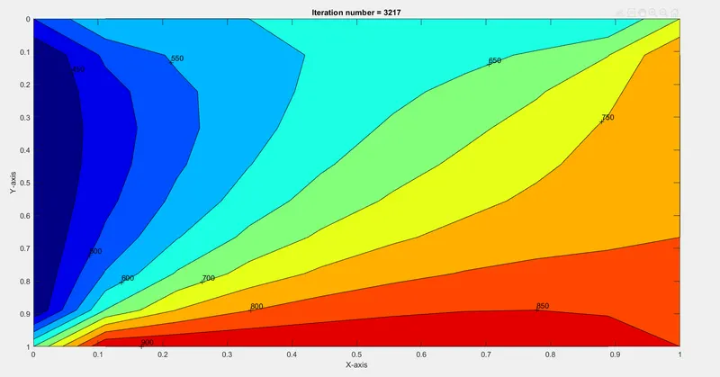
2. Gauss seidel
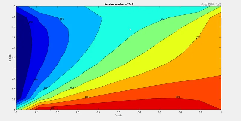
3. SOR method:
CONCLUSION:
1. Steady state analysis:
For steady state analysis, we can see that the SOR method had the fastest convergence rate followed by gauss seidel and then jacobian.
The SOR method reached convergence in just 29 iterations.
2. Transient state analysis:
2.1 Explicit:
In explicit solving, all the terms used in the formula were known to us therefore there was no need for iterative solvers there. We simulated the problem for 500 number of time steps.
2.2 Implicit:
In implicit solving, the SOR method had the fastest convergence rate followed by gauss seidel and then jacobian.