Week 3.5 - Deriving 4th order approximation of a 2nd order derivative using Taylor Table method

Aim: To derive 4th order approximation of the second order derivative using central, skewed right and skewed left sided difference method using taylor table method.

Procedure:

1. Central scheme method:

Number of nodes(n) = p + q - 1

where,

q = order of approximation = 4

p = order of derviative = 2

Therefore, n = 5

We need to take five node points within the numerical stencil.

Derivation:

`(del^2u)/ (delu^2) * (trianglex^2) = a*f(i - 2) + b*f(i-1) + c*f(i) + d*f(i+1) + e*f(i+2)`

• We need to calculate the value of all the constants.
• Using taylor series expansion for terms:

`a.f(i-2) = a[f(i) - (2f'(i)dx)/(1!) + (4f''(i)dx^2)/(2!) - (8f'''(i)(dx^3))/(3!) + (16f''''(i)dx^4)/(4!)]``

Just like this, we will expand all the given funtions in equation and for the taylor table for calculation.

	f(i)	`f'(i)(trianglex)`	`f''(i)(trianglex)^2`	`f'''(i)(trianglex)^3`	`f''''(i)(trianglex)^4`
`a*f(i-2)`	a	-2a	2a	-4a/3	2a/3
`b*f(i-1)`	b	-b	b/2	-b/6	b/24
`c*f(i)`	c	0	0	0	0
`d*f(i+1)`	d	d	d/2	d/6	d/24
`e*f(i+2)`	e	2e	2e	4e/3	2e/3
sum of coeff	0	0	1	0	0

• In order to solve the equation, we can use MATLAB and create a matrix to solve for the coeffiecient in the equation.

Matrix solution in MATLAB:

A = [1 1 1 1 1;
    -2 -1 0 1 2;
    2 1/2 0 1/2 2;
    -4/3 -1/6 0 1/6 4/3;
    2/3 1/24 0 1/24 2/3];
B = [0;0;1;0;0];

X = inv(A)*B; 

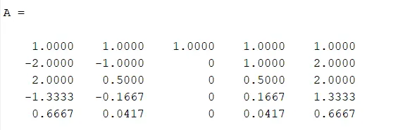
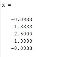
Therefore,

a = -0.0833

b = 1.3333

c = -2.5000

d = 1.3333

e = -0.0833

If we now re-write the equation with the values of constant, we get the common formula for 4th order approximations of the second-order derivative using central difference method.

`(del^2u)/ (delu^2) * (trianglex^2) = -0.0833*f(i - 2) + 1.3333*f(i-1) + (-2.5000)*f(i) + 1.3333*f(i+1) + (-0.0833)*f(i+2)`

2. Skewed right sided difference:

Number of nodes = p+q = 6

Therefore, we need to take 6 nodes using the numerical stencil.

`(del^2u)/(delx^2) * (trianglex)= a*f(i) + b*f(i+1) + c*f(i+2) +d*f(i+3)+ e*f(i+4) + g*f(i+5)`

• We need to calculate the value of constant to write the general form for skewed right sided difference.
• We will use taylor series to expand it and then for easier arrangement write it in taylor's table.

	f(i)	`f'(i)*(trianglex)`	`f''(i)*(trianglex)^2`	`f'''(i)*(trianglex)^3`	`f''''(i)*(trianglex)^4`	`f'''''(i)*(trianglex)^5`
`af(i)`	a	0	0	0	0	0
`b*f(i+1)`	b	b	b/2	b/6	b/24	b/120
`c*f(i+2)`	c	2c	4c/2	8c/6	16c/24	32c/120
`d*f(i+3)`	d	3d	9d/2	27d/6	81d/24	243d/120
`e*f(i+4)`	e	4e	16e/2	64e/6	256e/24	1024e/120
`g*f(i+5)`	g	5g	25g/2	125g/6	625g/24	3125g/120
Sum of coeff	0	0	1	0	0	0

• To solve this matrix, we will use MATLAB

A = [1 1 1 1 1 1;
    0 1 2 3 4 5;
    0 1/2 4/2 9/2 16/2 25/2;
    0 1/6 8/6 27/6 64/6 125/6;
    0 1/24 16/24 81/24 256/24 625/24;
    0 1/120 32/120 243/120 1024/120 3125/120];
B = [0;0;1;0;0;0];

X = inv(A)*B;
 

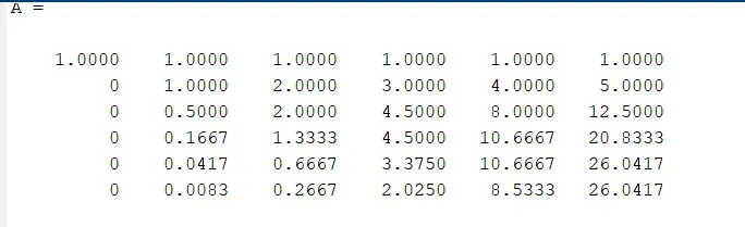
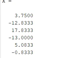
Therefore, we have the value of constants as

a = 3.7500

b = -12.8333

c = 17.8333

d = -13.000

e = 5.0833

g = -0.8333

`(del^2u)/(delx^2) * (trianglex)= (3.7500)*f(i) + (-12.8333)*f(i+1) + 17.8333*f(i+2) +(-13.000)*f(i+3)+ 5.083*f(i+4) + (-0.8333)*f(i+5)`

3. Skewed left-sided difference

Number of nodes: p+q = 6

Therefore, we need to take 6 nodes within the stencil.

`(del^2u)/(delx^2) * (trianglex)= a*f(i) + b*f(i-1) + c*f(i-2) +d*f(i-3)+ e*f(i-4) + g*f(i-5)`

• We need to calculate the value of constant to write the general form for skewed left sided difference.
• We will use taylor series to expand it and then for easier arrangement write it in taylor's table.

	`f(i)`	`f'(i)(trianglex)`	`f''(i)*(trianglex)^2`	`f'''(i)*(trianglex)^3`	`f''''(i)*(trianglex)^4`	`f'''''(i)*(trianglex)^5`
`g*f(i-5)`	g	-5g	25g/2	-125g/6	625g/24	-3125g/120
`e*f(i-4)`	e	-4e	16e/2	-64e/6	256e/24	-1024e/120
`d*f(i-3)`	d	-3d	9d/2	-27d/6	81d/24	-243d/120
`c*f(i-2)`	c	-2c	4c/2	-8c/6	16c/24	-32c/120
`b*f(i-1)`	b	-b	b/2	-b/6	b/24	-b/120
`a*f(i)`	a	0	0	0	0	0

• We can find the value of constants by forming a matrix in MATLAB

A = [1 1 1 1 1 1;
    -5 -4 -3 -2 -1 0;
    25/2 16/2 9/2 4/2 1/2 0;
    -125/6 -64/6 -27/6 -8/6 -1/6 0;
    625/24 256/24 81/24 16/24 1/24 0;
    -3125/120 -1024/120 -243/120 -32/120 -1/120 0];
B = [0;0;1;0;0;0];
X = inv(A)*B;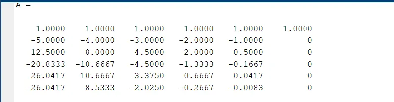

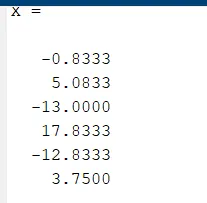
Therefore,

g = -0.8333

e = 5.0833

d = -13.000

c = 17.8333

b = -12.8333

a = 3.7500

Therefore, the general form for a skewed left-sided difference is

`(del^2u)/(delx^2) * (trianglex)= 3.7500*f(i) + (-12.8333)*f(i-1) + 17.8333*f(i-2) +(-13.000)*f(i-3)+ (5.0833)*f(i-4) + (-0.8333)*f(i-5)`

SOLVING FUNCTION USING MATLAB

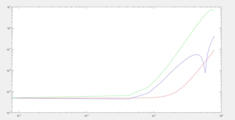
As the general form for 4th order approximations of the second-order derivative using central, Skewed right-sided difference and Skewed left-sided difference has been derived. We will use it to calculate the values of a function exp(x)*cos(x) and compare all the three by plotting a graph between them.

CODE:

1. Code for central difference:

function exit = central_difference(x,dx)

%function f(x) = e(x)*cox(x)
%analytical solution = second order derivation derived analytically
analytical_solution = -2*exp(x)*sin(x);


%central_difference: 
% (-0.0833)*f(i-2*dx)+(1.3333)*f(i-dx)-(2.5000)*f(i)+ 1.3333*f(i+dx)-(0.8333)*f(i+2*dx) 

central_difference = (((-0.0833)*((exp(x-(2*dx)))*(cos(x-(2*dx)))))+((1.3333)*((exp(x-dx))*(cos(x-dx))))-((2.5000)*((exp(x))*(cos(x))))+((1.3333)*((exp(x+dx))*(cos(x+dx))))-((0.0833)*((exp(x+(2*dx)))*(cos(x+(2*dx))))))/(dx^2);

exit = abs(analytical_solution - central_difference); 
end

2. Code for skewed right sided elements:

function exit2 = right_sided(x,dx)

%function f(x) = e(x)*cox(x)
%analytical solution = second order derivation derived analytically
analytical_solution = -2*exp(x)*sin(x);

%skewed right sided difference
% (3.7500)*f(i)+(-12.8333)*f(i+dx)+(17.8333)*f(i+(2*dx))+(-13.000)*f(i+(3*dx))+(5.083)f(i+(4*dx))
% +(-0.8333)*f(i+(5*dx))

right_sided_diff = (((3.7500)*((exp(x))*(cos(x))))-((12.8333)*((exp(x+dx))*(cos(x+dx))))+((17.8333)*((exp(x+(2*dx)))*(cos(x+(2*dx)))))-((13.0000)*((exp(x+(3*dx)))*(cos(x+(3*dx)))))+((5.0833)*((exp(x+(4*dx)))*(cos(x+(4*dx)))))-((0.8333)*((exp(x+(5*dx)))*(cos(x+(5*dx))))))/(dx^2);

exit2 = abs(right_sided_diff - analytical_solution );

end

3. Code for skewed left sided elements:

function exit3 = left_sided(x,dx)

%function f(x) = e(x)*cox(x)
%analytical solution = second order derivation derived analytically
analytical_solution = -2*exp(x)*sin(x);

%skewed left sided difference: 

left_sided_diff = (((-0.8333)*((exp(x-(5*dx)))*(cos(x-(5*dx)))))+((5.0833)*((exp(x-(4*dx)))*(cos(x-(4*dx)))))-((13.0000)*((exp(x-(3*dx)))*(cos(x-(3*dx)))))+((17.8333)*((exp(x-(2*dx)))*(cos(x-(2*dx)))))-((12.8333)*((exp(x-dx))*(cos(x-dx))))+((3.7500)*((exp(x))*(cos(x)))))/(dx^2);

exit3 = abs(analytical_solution - left_sided_diff);
end

4. Code for calling the functions:

clear all 
close all
clc

x = pi/3;
dx = linspace(pi/4, pi/4000, 20);

for i=1:length(dx)

    central_diff_error(i) = central_difference(x,dx(i));
    right_diff_error(i) = right_sided(x,dx(i));
    left_diff_error(i) = left_sided(x,dx(i));
end
figure(1)
loglog(dx, central_diff_error, 'r');
hold on
loglog(dx, right_diff_error, 'g');
hold on 
loglog(dx, left_diff_error, 'b');

RESULTS:

CONCLUSION:

• It can clearly be seen from the plot that central difference provides least error. This is due to the points taken within the numerical stencil. In central difference scheme the numerical stencil takes nodes close to the original point.
• Whereas in skewed right or left sided scheme, the node points taken are further from the original point showing a larger error.

Describe why a skewed scheme is useful?

• A skewed scheme is useful when we dont have information about the left and right side of the original point or when the point is at the boundary.

What can a skewed scheme do that a CD scheme cannot?

• If the original point is at the boundary, we will not be able to employ central difference scheme. Therefore, in such cases we need to use skewed scheme.